1. INTRODUCTION
Understandably, most people want less crime. Improvements to outdoor lighting are frequently mentioned in election promises, the news media and government planning documents as an option or action for crime reduction. Unfortunately, the common understanding of ‘improvements’ as ‘more and brighter’ in this context is likely to lead to ineffective or even counterproductive outcomes, as will be seen.
1.1 Rationale for this Study
Crime tends to be concentrated in cities, a fact that continues to attract the attention of criminologists (eg Glaeser and Sacerdote 1999, Ousey 2000)). Urban crime was already a problem before the widespread application of artificial lighting. This calls for an explanation as to why the present line of work has been pursued at all. The reasons are:
· It appears to be widely believed that more and brighter outdoor lighting would help to reduce both fear of crime and actual crime at night.
· Field experiments have been claimed as showing that increased outdoor artificial lighting does reduce actual crime.
· Publication of these claims reinforced existing beliefs, strengthening conflicts with separately established needs for environmental limits to outdoor lighting.
· In Part 1 of this work (Clark 2002b), study of the lighting and actual crime evidence indicated the claimed benefits were exaggerated or untenable.
· The facts uncovered went further than this, indicating that increased lighting and increased crime often occurred together.
· There are plausible mechanisms whereby the presence of light at night could facilitate some of the processes thought responsible for the growth of urban crime.
· Study of the nexus between outdoor lighting and crime now holds promise of containing the environmental as well as social problems of excessive outdoor light at night.
1.2 Results from Part 1
Part 1 of this work is a critical review of the literature on outdoor lighting and crime. It is summarised here as a foundation for this second part.
The literature indicates that artificial light at night may reduce the fear of crime to levels approaching those experienced in the same location in daylight. Illuminance of about 20 lux appears to be fully or highly effective in practice, and less is often adequate.[3] More light seems to be required in the presence of glare, or less without glare.
If there is some substance to the belief that more and brighter outdoor lighting would help reduce actual crime, then extending the belief to its ultimate stage means there should be little or no crime in the bright outdoor lighting conditions of daytime, but that is far from the facts. For example, 54% of violent crime in the USA occurred between 6 am and 6 pm, and only 20% of rapes involve unknown assailants at night (BJS 1999). Only 35% of all burglaries in the USA are reported to have occurred at night, or 48% of all burglaries for which the time of occurrence is known (UCR 1996). Note that these figures are for all reported crime in the whole of the USA, which gives them substantial face validity. In England and Wales, crime survey results indicated that nearly two-thirds of the total of assaults, burglaries, robberies, thefts and vandalism occurred after dark (Ramsay and Newton 1991, ONS 2000). An unresolved issue is the extent to which the proportion of crime at night is influenced by effects of light at night rather than by other factors such as the available amount of leisure time at night.
Effects of light on actual crime have been investigated with field studies, but extraneous influences have often confounded the results. Crime-reducing, nil, uncertain, and crime-increasing effects of light at night have variously been reported for night or day or both. Thorough scientific reviews published in 1977 and 1997 in the USA concluded that the effect of lighting on actual crime was unknown. Nevertheless, crime prevention specialists and some academics have asserted that lighting is important, at least in some circumstances, in the fight against crime. Recent UK findings of beneficial effects of brighter lighting have bolstered this view despite complaints, by others, of procedural and analytical shortcomings in the studies.
Part 1 indicates that, in general, lighting and crime experiments have not been planned and executed well enough for the results to be considered reliable. There is evidence of systematic bias towards a beneficial effect of lighting on crime. Industry and company funding is known to be associated with an unjustifiable excess of findings beneficial to the industry or company concerned. In some or even the majority of cases, areas with substantially elevated crime incidence (crime hotspots) have been chosen for experimental treatment. Regardless of how ineffectual the treatment might be, reduced crime afterwards relative to control areas is naturally more likely and the increased lighting tends to get the credit for the beneficial result. Pooling results to get apparently greater precision and reliability does not eliminate such systematic bias. Results obtained by an instance of this method were shown to be improbably large, given the possibility that the experimental treatment could be repeated many times, with claimed crime reductions for each treatment compounding to values far lower than have ever been observed. The main conclusion of Part 1 is that increased outdoor lighting has not been shown to have a reliably beneficial effect in reducing crime.
Marchant (2003) examined the statistical methods used in the Dudley and Stoke-on-Trent lighting and crime experiments and in the meta-analysis described in Part 1. He found several errors that were serious enough for the conclusions of these studies to be rejected. This is independent support for the writer’s findings about these studies, and it strengthens the case that the main conclusion of Part 1 is correct.
Strident campaigns based on the apparently erroneous results have encouraged public lighting projects for crime prevention in the last few years, especially in the UK. Street crime in the UK rose by 28% in the year ending in April 2002 (Hoge 2002).
New terminology was defined in Part 1 to assist in understanding the lighting and crime relationship. By its direct physical effect on visibility, light may aid or hinder criminal acts at night at the time of actual or intended commission. Examples are seeing where to break in, and being seen breaking in. Indirect effects of light act through intervening social factors, generally with time delays, and may influence crime by day as well as at night. Existing mainstream use of the term positive correlation is retained for the case where increased lighting is associated with increased crime. The contrary use sometimes found in the crime prevention literature is avoided in this work. The terms ‘adverse’ and ‘beneficial’ are used here as they are unambiguous.
2. GROWTH IN LIGHTING AND IN CRIME
Whatever the relationship, if any, between outdoor lighting and crime, it seems reasonable that the way these and related quantities have varied over the last century or more should be known and understood as a highly desirable precondition for studies of the present situation. As it happens, the required historical data tend to be sparse, beset by discontinuities and other inconsistencies, and difficult to track down. For many countries, the records for recent years are hardly any better, if they exist at all.
For periods of up to a year or so used to date in the ‘before’ and ‘after’ phases of the field-based studies reviewed in Part 1, it appears that relatively small increments in outdoor lighting have not been reliably demonstrated either to decrease or increase actual crime. Here, changes occurring over much longer intervals in lighting and crime are examined.
Ramsay and Newton (1991, p 12) commented on the steep rise in crime in the UK following WW2 while major street lighting improvements were taking place. As they put it, this “scarcely suggests that street lighting improvements are of great importance in preventing crime”. The co-occurrence of the increases suggests more than this, viz that there is a positive (ie adverse) correlation between lighting and crime. If there is a persistent correlation, then it could be useful to know why.
Others have noticed that urban crime rates and outdoor lighting both increased substantially during the twentieth century. Perhaps the notion of a connection has been dismissed each time at the outset as contrary to common knowledge that lighting reduces crime, and therefore fanciful. Regardless, the issue seems to be worth another look now that the best short-term studies have been exposed as rather inconclusive or unconvincing. Time-series measures of lighting and crime need to be examined for evidence of association and causality. Availability of reliable data determines how far back such assessments can be taken. Here, attention is limited to periods starting at least a decade after the initial introduction of electric lighting.
Many older people are able to recall that their childhood hometown skies had far more stars than is now the case. There is no doubt that their loss is a result of a great increase in outdoor lighting, but it is also important to know how this change has progressed. If the forms of long-term increase for lighting, crime and other potentially important factors such as the economy are sufficiently different, it may allow disentangling of possible causality.
2.1 Outdoor Lighting
2.1.1 Brief history
Prehistoric campfires provided warmth, light and a degree of safety at night against attack by wild animals. The flames doubtless acted also as beacons for late-returning hunters and, rather less beneficially, for hostile warriors from other tribes.
Fixed urban outdoor lighting at night was instituted in Paris of the 1660s by Louis XIV as a supposed crime prevention measure (D’Allemagne 1891). Candles gave way to oil lamps in the eighteenth century, and coal-gas lighting was introduced in London in 1809. Principal street intersections in Los Angeles were first lit by the Los Angeles City Gas Company on 1865-04-14. Edison’s incandescent carbon-filament light bulb was invented in 1879. These lamps and the electrical system to supply them were first marketed in New York in 1881, with safety as a selling feature. The first electric streetlight[4] in Los Angeles became operational on 1882-12-31 (Anon. 2002a). However, it was not until the metal filament displaced the carbon filament in the 1910s that artificial light had become sufficiently bright and affordable to start having a broad impact on outdoor activities at night.[5]
Public lighting increased greatly during the twentieth century, not only in terms of the area lit but also in the strength of illumination. For example, in an Iowa town in 1895, public artificial lighting was not required between midnight and 5 am and not at all if there was enough moonlight to see by (IDA IS114 1996), say about 0.1 lux. Between 1925 and 1996, the recommended average for street lighting in the USA went from 3 lux to 14 lux. On this sparse indication, the illuminance of outdoor lighting increased by a factor of 140 times over a century. If the growth rate in this time had been uniform, it would have been an increase of about 1.6 times per decade. Note that this takes no account of the growth in the area illuminated.
In many countries, past records of extent, use and total energy consumption of outdoor lighting seem to be limited or no longer in existence. Some historical records of electrical power generating capacity are extant (eg Hirsh 1999) but the energy fractions used for outdoor lighting, let alone the quantity of indoor lighting contributing to outdoor ambient illumination, appear far less likely to be available with the degree of regional detail and continuity required for research purposes.[6] In Australia, the inadequacy of even relatively recent records became apparent when compliance with the Kyoto Protocol was first being considered. It took some years for the government authority involved to publish total electrical energy usage for the 1990 base year of the Protocol. The outdoor lighting component for 1990 still does not appear to be available from this source, let alone for earlier years. Government departments in the UK are likewise unaware of basic facts about the amount of energy used and wasted by outdoor lighting (CPRE 2003 p 17).
Presumably, the preservation of energy use details for outdoor lighting over decades has not been seen as a priority let alone a necessity in the industry. The situation appears to have deteriorated further with the trend in some countries, including Australia, for government-owned electricity utilities to be privatised. Neglect is bad enough, but on top of this, the continued survival of industry records of previous lighting systems and energy usage seems to be at risk when community and environmental groups seek to quantify their complaints about obtrusively relit commercial premises or sports grounds, or about larger-scale developments.
Regardless of the apparent dearth of useful numerical data on the growth in total light radiated by outdoor lighting during the course of the twentieth century, there is no doubt that outdoor lighting has grown from virtually nothing to the present unprecedentedly large values. As a more or less constant minimum proportion of a city’s total outdoor light flux is scattered by the atmosphere back towards any particular point on the ground (eg Fisher 1993), measurements of this light (artificial skyglow) are a valuable independent source of information about the rate of change in the total amount of light in the city.
The absolute quantity of light radiated upward at any time can also be derived from skyglow measurements at that time or vice versa, albeit with a lot more effort (eg Garstang 2000a, Falchi and Cinzano 2000). Periods in which observational data are of poor quality or non-existent can be dealt with satisfactorily by interpolation, assuming monotonic growth tied to the known initial and observed recent values. This is especially useful for periods covering the introduction of electric lighting as the natural skyglow value is reasonably well quantified and the initial artificial skyglow value is effectively zero.
Incandescent lamps and their quartz-halogen derivatives are still in common use for outdoor lighting although increasingly they are being supplanted by lamps using an electrical discharge in low- or high-pressure gas. Relative to incandescent lamps, these newer types tend to be between four to ten times better in turning electrical energy into light (eg IDA IS115 1998). The successive introduction of improved lamps must have caused the total amount of outdoor light flux to grow more quickly than the growth in electrical energy used for making this light (eg Cinzano 2000d, Hänel 2000). The development of solid-state light sources has now reached the stage where they also are increasing the range and affordability of outdoor lighting, thereby further promoting the use of artificial light at night.
Historically, motivating factors that have led to more and brighter outdoor lighting include:
· facilitating pedestrian mobility and vehicular traffic at night by reducing the likelihood of accidents and aiding wayfinding,
· allaying the fear of crime at night,
· attracting individuals to commercial venues such as bars, theatres and shops,
· the increasing popularity of outdoor sports at night for players, spectators and television audiences,
· individual, corporate or national self-interest or self-aggrandisement, as with bright lighting of power stations, illuminated advertising and architectural floodlighting,
· increasing luminous efficacy of lamps, giving more light for the amount and cost of the power consumed,
· safety and productivity in outdoor industrial operations at night,
· promotional incentives by operators of thermal power stations to meet the base load required at night for profitability, and
· as an intuitive countermeasure to actual crime.
General experience is that results seem to confirm expectations. In some cases, especially the last two or three, however, most individuals have neither the analytical skills required nor access to quantitative data to make reliable judgements of the effectiveness of outdoor lighting. As indicated in Part 1, even the experts have difficulty in the case of actual crime.
Regardless, many practitioners of Situational Crime Prevention[7] appear to believe that more and brighter outdoor lighting at night does reduce crime, and often recommend increased lighting accordingly. The belief has permeated academia to the point where discordant evidence has caused surprise.[8]
2.1.2 Indications of growth in lighting
Pike (1976) and Berry (1976) reported skyglow growth in southern Ontario as about 7% to 10% a year. A steady rate of growth gives an exponential increase.[9] Cinzano (2000d) summarised observations in southwestern USA: 5% to 6.2 % per year increase over San Jose from 1948 to 1978, and 10% to 15% per year over Tucson prior to 1972. Shaflik (1997) referred to International Dark-Sky Association material that put the growth rate for artificial skyglow over some American cities at 30% per year (14 times per decade). For Akita City in Japan, the increase from 1993 to 1996 (Isobe and Hamamura 1998) was 16% per year, equivalent to 4.6 times per decade. Van den Burg (2000, p 33) quoted what appears to be a decadal increase of 15 times in skyglow over The Netherlands.
Cinzano (1995) summarised measurements of the astronomical V-band brightness of the night sky at Asiago in northern Italy: the value in 1993 was “at least doubled with respect to the sixties.” The V-band measure is effectively made with light passed through a green filter and is approximately proportional to luminance.[10] Allowing for the presence of natural skyglow in the measure would indicate more than a doubling in the artificial component. Since then, Cinzano (2000d, 2002) has produced a graph of Italian observatory measurements of artificial skyglow from 1960 to 1994. The trendline appears to be exponential with a decadal growth rate of about 2.6, representing an annual growth of 10% or a factor of 45 times over 40 years. For Italy overall, exponential growth in the artificial component at sea level from 1971 to 1998 was typically 7% to 10% a year (Cinzano, Falchi and Elvidge 2001b) or 2.0 to 2.6 times per decade.
A decade of satellite measurements of optical energy radiated from Earth’s populated areas (Cinzano, Falchi and Elvidge 2001a)appears to indicate a generally exponential growth of skyglow. Worldwide, only a few areas such as central India and some cities in Russia have shown a reduction in upward light emissions in recent years (NASA 2000, Sutton 2002). Satellite data for 1993 to 2000 has been analysed to determine that the total skyglow over the UK increased in this time by 24% (CPRE 2003).
2.1.3 Skyglow, outdoor lighting and population
With a moonless clear sky and well into the dark hours, the absolute values of both natural and artificial skyglow are dependent on geographical position and direction of observation. For the present purpose, the exponential growth in the artificial component added to the value of the natural component is a key issue. The luminance of the natural component varies according to the phase of solar activity. Garstang (1989a) used 53.7 nanoLambert (nL) (171 µcd/m2, or 0.171 mcd/m2) as the minimum, occurring at solar activity minimum, and 55 nL for the same quantity in Garstang (2000). Cinzano (2000d) allowed a 1 stellar magnitude[11] increase over the minimum natural skyglow at solar maximum, which would give a value of 0.43 mcd/m2 and a logarithmic mean of 0.27 mcd/m2. The value used by Cinzano, Falchi and Elvidge (2001b) as typical was close to the latter. The amount of artificial skyglow in remote rural areas can still be much smaller than the minimum natural value. In the total skyglow over large cities, however, the natural component, even at its maximum, generally became negligible decades ago.
Walker’s law (eg Garstang 2000; Mizon 2002, p 65) is an empirical relationship for predicting the artificial component of sky luminance at 45º above a city with known characteristics at a known distance. A simplified version of the law is based on the assumption that the amount of outdoor lighting per member of the population is a constant. Astronomers such as Pike (1976) once hoped it to be so, but time has shown that this factor has continued to increase. Pike’s pioneering work on modelling skyglow growth in southern Ontario during the 1970s provided indications even then that the growth was exponential. His predictions about the Milky Way being blotted out in southern Ontario by 2000 have unfortunately proved correct.
Garstang (1991) calculated the effect of airborne dust on skyglow. Desert dust and volcanic dust have closely comparable effects. Dust below about 10 km altitude reduces skyglow and higher dust increases it. For the present purpose, the effect on skyglow is unimportant. The same conclusion applies to Los Angeles smog (Garstang 2000), so the effects of dust and smog generally can be ignored in this document.
Garstang (2000) calculated the growth of skyglow over Mount Wilson Observatory in California from 1910 to 1990 using a set amount of light flux emission (1000 lumen) per person from 124 cities in the Los Angeles basin. As in earlier papers, Garstang chose to exclude effects of changes in lighting technology, not because they were unimportant but to give a simpler basis for comparison of results. Within a large margin, the results were consistent with a few visual observations of stellar limiting magnitudes. The plotted curve overall is concave upward, but not to the extent implied by the actual observations of skyglow elsewhere in southwestern USA reported in the preceding section. Garstang (1989a) did consider introducing a factor to give faster skyglow growth than with population alone, but tested for this and considered that there was insufficient evidence to support it.
To estimate the threat of skyglow to national parks, Albers and Durisco (2002) calculated skyglow over the contiguous states of the USA. They also assumed that cities emit light in proportion to population. The resulting map looks like a satellite image of real city lights at night, but the calculated intensity of city centres appears deficient[12] and some cities look to be fainter than they are in satellite images. The second of these differences probably arises because the light emission per person in the USA does differ substantially between cities (see Section 5.2). Garstang’s calculation for Mount Wilson would tend to ‘average out’ the local variations.
Assuming that skyglow is a linear function only of population ignores the long-term increase in public lighting illuminances mentioned in Section 2.1.1. It also ignores the increasing amounts of light being used by retailers and advertisers, and the increasing use of decorative and security lighting. The amount of light produced for a given amount of electrical energy has risen with improvements in lamps. Because electricity has tended to become more affordable over the years, the amount of light provided for a given inflation-corrected cost of electricity has increased even more. All of this suggests that the outdoor luminous flux per person has been growing substantially. If city area grows linearly with population, then artificial skyglow can be expected to grow in proportion to city area multiplied by mean illuminance. Even if the time rates of increases in area and illuminance are both linear, the product of these is exponential.
2.2 Crime Data
Crime appears to have increased substantially in many countries during the twentieth century. Criminological studies of long-term variations in the crime rate (eg Graycar 2001) and its causes are hampered by factors such as:
· large shifts in what society regards as a crime (eg drunkenness, nude bathing, homosexuality),
· the emergence of new crimes (eg Internet fraud, aircraft hijacking),
· political and industrial influences on reporting and recording of crime and its solution rates,
· improvement in methods of detection and prosecution of offenders, and so on.
The problems of poor data quality and inadequately standardised crime definitions have been known for over a century but are still being dealt with. Differences in criminal justice systems add to the problems of comparing international crime rates (eg Barclay and Tavares, 2000). Regardless, there are often inexplicably large differences between countries in specific crime rates, eg homicide (Graycar 2001).
The following sections present within-country comparisons of available lighting and crime growth data.
2.3 Growth in Lighting and Crime in Individual Countries
2.3.1 Australia
Despite substantial effort, the writer did not find suitable records of energy use for outdoor lighting in Australia and the proportions of various lamp types installed. The same applies to records of illumination levels or total light output, so recourse has been had to astronomical observations.
For the period 1880 to 2001, artificial skyglow values shown in Figure 1 (all of the figures are grouped at the end of this document) have been inferred from limiting unaided visual stellar magnitudes assembled by the writer from observations in recent decades from Melbourne suburbs plus a few more as far back as the mid-1950s (reported in Dudley 2000). Fluctuations must have taken place during social upheavals such as the Great Depression and the two World Wars, especially WW2 because a blackout was enforced,[13] but they are not shown because of the absence of specific data for the years in question. The skyglow changes caused by population changes at those times were small in the USA (Garstang 2000), but social, economic and technological effects on skyglow could well be larger than the population effects. The sky reference area chosen for skyglow observations and calculations is at 45 degrees altitude, due south of an observing site about 11 km northeast of the Melbourne central business district. The zenith might have been a better reference position, but this is relatively unimportant for the present purpose.
The pre-electric-lighting ordinate of the skyglow curve in Figure 1 is 0.27 mcd/m2, typical of the luminance of the natural clear moonless night sky. For the luminance of the Melbourne sky to start at that value and to be where it is now and where it has been in recent decades is most readily explained if the growth rate of the artificial component is taken as exponential. The observed increase is close to doubling in each decade.[14] To sufficient accuracy for the present purpose, the skyglow luminance S mcd/m2 is given by
S = 0.27 + 0.00189*2^((year-1880)/10).
On the basis that there do not appear to have been large changes overall in the shading of installed outdoor light fittings against upward light spill in recent decades and that probably only small changes have occurred in the amount of light reflected upward from the terrain, the plotted skyglow curve in Figure 1 is considered to indicate how the total of artificial ambient light outdoors at ground level has grown in recent decades over the more densely populated areas of Australia. The growth rate has probably been greatest in the state capital cities, and slowest in rural areas. Determining the actual lighting growth rate in rural areas using skyglow observations is complicated by the additive effects of waste light from distant cities and nearby towns. Examples of this are given by Berry (1976), Cinzano (2000c,d) and Dudley (2000). Note that luminance, rather than log luminance, is additive.
The form of the skyglow curve in Figure 1 can reasonably be supposed to be typical for most of the highly urbanised Australian population. Of course, long runs of frequent observations of skyglow in various locations would be better to work with, but so far, few Australian skyglow observations seem to have been published.
Figure 1 also shows three sets of Australian recorded crime data. These data were selected on the basis of being available, appropriate and freely accessible through the Internet for ease of checking and comparing by others.[15] Data for homicide were also available but not included as the rate has not varied greatly over the whole century[16] (Graycar 2001). The numbers for homicide are so small relative to those for other crimes that they would make no practical difference anyway in any overall number or rate. For the crime data that are shown in Figure 1, partition into day and night occurrence would be valuable but such data did not appear to be available, either on the Internet or elsewhere.
The yearly crime rate data for 1974 to 1992 are from Walker (2002), for 1993 to 1999 from Graycar (2001), and for 2000 and 2001 from ABS (2003). The usual basis of reporting crime rate per 100 000 of the population has been changed proportionally to smaller population numbers for convenience in plotting the data with a common ordinate scale.[17] The data are not quite internally consistent and seamless because of evolving differences between state and territory jurisdictions in definitions of crime, late numerical corrections and other relatively minor perturbations. For example, data included as Burglary are called Unlawful Entry with Intent in two of the source documents. These shortcomings again appear to be of little consequence for the immediate purpose.
Part or all of the drop in motor vehicle thefts in the 1990s appears to have been a result of various measures stemming from political concern, such as increased attention to insurance fraud, vehicle ‘rebirthing’ and anti-theft devices (eg Grabosky and James 1995, Section 14).
The Australian population is also plotted in Figure 1 using data from Lahmeyer (2002). Missing data for some early years have been interpolated. Population data are shown because they are readily available and because many of the social factors that might be thought to encourage crime (eg housing density) seem likely to be related to the size of the national population. Given the different character of the skyglow and population growth curves, it was thought possible that correlations of each with crime data might indicate any relative differences in degree of association.
Australian crime records are available for six of the years in the period 1890 to 1902, but they are given only as offences against the person and offences against property. Public drunkenness is not included here as it is no longer a crime. The total rate of violence and property crime for this period in Australia fell from about 11 per 1000 to under 7 (Graycar 2001). A roughly equivalent total rate of violence and property crime in the last years of the twentieth century is over 60 per 1000, ie about 7 times greater. The total rate for all crime in Victoria was about 40 per 1000 in the first half of the twentieth century, doubling from 1945 to 1955 and trebling by 1975, reflecting an Australia-wide pattern (Walker (2002), hard copy version cited by DCPC (2002) p 11).
Over the twentieth century, the Australian population grew by a factor of about 5. The increase in natural plus artificial outdoor light flux in the Melbourne metropolitan area in that time is about 30 times, less if moonlight is included in the natural flux, or more if moonless overcast nights are considered. It is more again if the peak ambient illuminance in large city centres is considered, or less for the typical ambient illuminance in the outer suburbs. Crime rate growth (day plus night) is obviously correlated both with lighting growth and with population growth over decades. Neither appears to be a markedly better correlate than the other.
Discussion of causality would be premature at this stage. Readily available Australian crime data appear to be of insufficient quantity and quality to get much further with this line of investigation. In the absence of reliable crime data for the earlier part of the twentieth century, attention has been directed to other countries with better records.
2.3.2 England and Wales
Population data for 1900 through 1997 from the House of Commons library (Hicks and Allen 1999) for England plus Wales are plotted in Figure 2. The population graph was extended by linear extrapolation back to 1898 and on to 1998. Total crime data from the Home Office (2002b) for 1898, 1899, and to 2001 (retaining the pre-April 1998 counting rules) have also been used to extend the graph. The crime data set covers a much longer span than that for Australia in Figure 1.
Actual historical data for the growth of skyglow in England and Wales would be ideal to include in Figure 2, but not even the world’s first book in English about light pollution (Mizon 2002) includes this despite its UK origin.[18] Nor were any quantitative records found in Internet and literature searches until May 2003, when the CPRE (2003) analysis of satellite data provided an exponential growth rate for overall light pollution from the UK: 24% for the 7 years from 1993 to 2000. As an exponential rate, this is equivalent to a 3.12% growth per year or 36% in a decade.[19] To derive the skyglow growth curve for the UK starting from the 1890 natural skyglow value of 0.27 mcd/m2, exponential growth was assumed, with the value at 2000 set equal to that used in Figure 1, ie 8.0 mcd/m2, corresponding to medium light pollution with about 3% of the naturally visible stars still visible. To sufficient accuracy for the present purpose, the total skyglow S mcd/m2 is given by
S = 0.5*1.03121^(year -1910).
This growth curve is shown in Figure 2. It is intended to be representative of the sky seen from a suitable location near any UK city or large town. The lack of account of the war blackouts and the 1930s depression detracts somewhat from its usefulness. Fortunately the scale of the skyglow curve is immaterial in ordinary correlation calculations. The shape of the curve is of more importance. As can be seen in Figure 2, its upward concavity tends to match the long-term trend of the police-recorded indictable crime rate in England plus Wales.
In Figure 2, the crime rate since 1989 appears to be a combination of reasonably steady growth plus an increment peaking in 1991 or 1992. In following sections, this feature will be seen to have approximate counterparts in several other countries. The subsequent decline back to the long-term trend may have been due entirely to change in the unknown factors that produced the increment (eg fluctuations in the supply of illicit drugs?), but the Home Office (2002a) treated the period of the decline in isolation in attributing the decline partly to the contribution of police and their partners in crime control. This is not to deny the value of police or of outcomes of the Crime and Disorder Act 1998 but is a reminder of the difficulties of interpreting short runs of time-series data.
2.3.3 USA
By itself, the existence of good correlations between lighting and crime in Australia and in England plus Wales is not sufficient to justify international generalisations from these national findings. Criminologists caution that international comparisons of crime rates can be misleading (eg Barclay and Tavares 2000). Direct comparisons from 1981 to 1996 between crime data for the USA and England plus Wales (Langan and Farrington 1998) indicate that there are substantial differences between the respective rates and trends for specific crime types. Therefore it is important to extend this investigation to other countries. The USA is a readily justifiable choice because of the apparent wealth of US crime data readily available online, some of it even dating back to 1860 for cities (eg Monkonnen 1994).
Unlike the situation in England and Wales, however, usable crime data for the USA spanning the twentieth century were not found. Most of the available time-series data for US crime only covers recent decades. Inspection of Bureau of Justice Statistics data starting in 1973 (BJS 2002a) indicated that correlations of surveyed property and violence crime rates with skyglow and population would be small or negative. However, correlations with recorded violent crime and arrest rates still appear to be positive.
Annual crime rate data for the USA from 1960 are given by Maguire and Pastore (2002, Table 3.120), based on BJS Uniform Crime Reports (UCR) data. For years 1933 to 1959, the source was JRSA (2000). The total of property and violent crime rate, including homicide, is called the Total Crime Index or the Index Crime Rate, shown in Figure 3. The discontinuity at 1959 is an artifact resulting from change to the dollar limit for larceny. The 2001 results (Butterfield 2002) are not shown in the figure: the UCR rate increased by 2.1 % over the 2000 value, ending the ten-year decline. During 2001, robberies climbed 3.7 percent, burglaries 2.9 percent, petty thefts 1.5 percent and motor vehicle thefts 5.7 percent.
No regional or national skyglow data were readily available so the skyglow curve used in Figure 1 is used again as representative of exponential growth of skyglow near cities. US population (Demographia 2002), the combined adult and juvenile estimated drug arrests rate (BJS 2002a) and the total US federal and state rate (BJS 2002a) are also included in Figure 3. The incarceration rate was included as it could possibly account for at least part of the reduced growth or falling trend of crime in the US while the various factors conducive to crime presumably continue to increase.[20], [21] Over half of the steep increase in US prison population since 1990 is a result of convictions for violence.
Drug offences were included in Figure 3 as an exception to the flatter trends for most other crime in the US over recent decades. All or most of the difference in growth rates may well be caused by factors other than any effects of lighting. At first sight there might seem to be no good reason to expect any direct connection at all between lighting and drugs crime. However, exposure to artificial light at night already appears to have reached levels great enough in some cases to reduce the production of melatonin by the pineal gland (see Section 6.1.4 below). This is so both in the evening and then later in the small hours when this part of the human endocrine system appears to be most sensitive to small amounts of light.[22] If drug taking is indeed somehow affected by endocrine disruption as an explanation of the differences between drugs crime and other crime in Figure 3, this would not necessarily affect the relative day-to-night ratio for particular kinds of offences.
2.3.4 Canada, New Zealand and other countries
Recorded crime data from 1962 to 2001 are available for Canada (eg Statistics Canada 2001). Variations in the Total Criminal Code rate appear to mirror those in the US Total Crime Index shown in Figure 3, although the ordinates are higher. The recorded overall offence rate for New Zealand for years 1970 to 2001 (Statistics NZ 2002) has a somewhat similar shape and ordinates a little higher again. Note that crime rate differences between countries are not a reliable guide to relative inherent criminal tendencies because of confounding by differences in laws, policing and justice procedures, statistical treatments and other relevant factors (eg Barclay and Tavares 2002). Therefore, international differences in any environmental influences on crime should not be inferred from such crime rate differences.
The United Nations has collected annual total recorded crime rates for 88 member countries (UN 2000). The years covered are 1980 through 1986 and 1990 through 1997. Most of the responding countries have not provided data for all of these years. In several cases, the data are obviously incorrect or unreliable, with non-credible minuscule values or massive changes from one year to the next. Political instability and adverse consequences of war seem likely to have led to some of the effects.
National data were selected from the UN table with the following criteria: data runs had to cover at least 12 years apart from the three-year gap from 1987 through 1989. In one case, Argentina, missing data for 1993 and 1994 were estimated by linear interpolation between 1992 and 1995. All missing data for 1987 through 1989 were estimated by linear interpolation. Countries with apparently incorrect or unreliable data were excluded, unless the problem was a single typographical error such as a factor of 10 in one entry for Japan. Small countries were not included, nor were the five countries already considered (Australia, Canada, England plus Wales, New Zealand, and the USA). This left 15 countries. Their data are shown in Figure 4. All show a positive gradient overall. The mean linear increase in crime is 4.5% per year (range 1.08% to 11.3%). This is a factor of about 1.5 per decade. The crime growth rates in the five countries already considered are less than half of this. Nevertheless, it does indicate that any association between artificial light at night and crime does have global applicability instead of being confined to, or most active in, countries with some common feature, such as English as the principal language.
2.4 Correlations Between Crime and Other variables
Linear correlation coefficients calculated for the crime and justice data in Figures 1 to 3, and for similar data from Canada and New Zealand, are shown in Table 1, below in this section. The values are generally high but do not indicate a consistent superiority for either lighting or population as a correlate with crime. The balance seems to shift a little towards lighting if crime and justice numbers are used instead of rates. The change to numbers can be achieved by multiplying rates by population. This has the same effect on correlation coefficients as leaving the rates as they are and dividing skyglow by population, which gives a variable proportional to the amount of outdoor artificial ambient light per person. This variable is mentioned again in Section 5.2.
It seems unlikely that the picture presented by these correlations would change much in either direction if data for more of the whole century became available. By inspection, Garstang’s population-based California skyglow growth data would appear likely to give correlation coefficients with crime similar to those for the population. Garstang’s data were not included in the figures or in Table 1 because the observational evidence for exponential growth is so strong.
Hays (1970, p 565) stated, “There is no guarantee that all psychological relationships of theoretical or applied interest must be linear in form.” The logarithm of light flux might be a more suitable variable to investigate for linear correlation, given that the visual system tends to respond to light in a logarithmic fashion, and given the apparent exponential nature of existing growth in artificial skyglow. Hays (1970, p 563) indicated that using the logarithm of an exponential quantity in this way is appropriate. The correlation coefficients of the various crime and justice data, and population, with log skyglow are therefore included in Table 1. Simple counts indicate that these log skyglow correlation coefficients with crime and justice data are most often the highest values across the three columns. The small numbers and partly overlapping data sets deter a formal significance test but future work might be better organised to deal with this issue. Not surprisingly, population correlates better with log skyglow than with skyglow in 4 of the 5 cases in Table 1.
A further caution seems worthwhile about the relative amounts of crime in the countries studied. The crime data are from police records. Crime surveys in 14 countries indicated rather different relativities, and also revealed a latitude effect- colder countries tended to have lower crime rates (Walker, Wilson, Chappell and Weatherburn 1990). However, it is the rate and direction of change of crime, and of artificial lighting, with time that are of most interest here, rather than the absolute scales of crime and lighting.
It might seem rather naïve to expect total crime to correlate strongly with lighting, given that crime was problem long before bright lighting became widely available or used[23] (eg Sharpe 2002). Therefore, it might appear more reasonable to use the increment in crime above some pre-lighting base crime rate as a variable in looking for lighting and crime correlations. Subtracting a constant base rate from any of the crime data does not change linear correlation coefficients, however. Likewise, it is almost immaterial in this context whether total skyglow or just its artificial component is used. The correlations shown in the table are a reasonable guide as they stand. The squares of the correlation coefficients have been included to indicate the proportions of variance in crime and justice data explained by skyglow and population.
Correlation studies rate a mere 1 on the Scientific Methods Score used by Sherman, Gottfredson, MacKenzie, Eck, Reuter and Bushway (1997), but that is in the context of experimental hypothesis testing rather than exploratory analysis of complex systems. The correlation studies used here are quite appropriate for guiding hypothesis formulation. Furthermore, the data sets used in this case are massive, applying to national populations over three to ten decades.
TABLE 1. Correlations of Crime, Justice, Population and Skyglow
|
|||||
|
Country |
Quantity: Crime Rate, Justice Rate, or Population |
Inclusive
From To |
Linear Correlation Coefficients r (above, r2 below) with |
||
|
Skyglow
|
Log Skyglow
|
Population |
|||
|
Australia
|
Motor Vehicle Theft |
1974 2001 |
0.626 0.392 |
0.759 0.576 |
0.770 0.593 |
|
Robbery |
1974 2001 |
0.985 0.970 |
0.945 0.893 |
0.937 0.878 |
|
|
Burglary |
1974 2001 |
0.873 0.762 |
0.953 0.908 |
0.954 0.910 |
|
|
Population
|
1890 2001 |
0.858 0.736 |
0.988 0.976 |
1 1 |
|
|
England plus Wales
|
Indictable Crime |
1898 2001 |
0.970 0.942 |
0.870 0.757 |
0.826 0.682 |
|
Population
|
1898 2001 |
0.899 0.808 |
0.995 0.989 |
1 1 |
|
|
USA
|
Recorded Total Crime (UCR Index) |
1933 2001 |
0.683 0.466 |
0.895 0.801 |
0.913 0.834 |
|
Recorded serious violent crime (not shown in Figure 3) |
1973 2001 |
0.622 0.387 |
0.764 0.584 |
0.750 0.569 |
|
|
Estimated Total Drug Arrests |
1970 2001 |
0.926 0.857 |
0.926 0.857 |
0.925 0.856 |
|
|
Incarceration, Federal plus State Prisons |
1980 2001 |
0.980 0.960 |
0.995 0.990 |
0.995 0.990 |
|
|
Population
|
1900 2001 |
0.989 0.978 |
0.999 0.998 |
1 1 |
|
|
Canada (Not shown in figures) |
National Criminal Code Rate |
1962 2000 |
0.626 0.392 |
0.821 0.674 |
0.808 0.653 |
|
Population
|
1890 2001 |
0.835 0.697 |
0.821 0.674 |
1 1 |
|
|
New Zealand (Not shown in figures)
|
Overall Offence Rate |
1970 2001 |
0.758 0.575 |
0.889 0.790 |
0.824 0.679 |
|
Population
|
1970 2001 |
0.980 0.960 |
0.983 0.966 |
1 1 |
|
For each of the three countries studied in Figures 1 to 3, real expenditure on police has increased over recent decades. For example, allowing 1.726 for the total inflation, the real per capita expenditure increase for all US police forces combined over the period 1980 to 1999 (BJS 2002b) was a factor of 2.016. The bulk of this expenditure is likely to have gone into increasing police numbers rather than into more and better equipment and training (Greenberg 1983).
Doubling of police numbers represents a compounding 10% increase repeated about 7 times. Using Marvell and Moody’s (1996) estimate of the effect of a 10% increase in police numbers, a doubling of police would reduce crime to (0.971)7 , ie 0.814, or a reduction of 18.6%. Goodman’s (2002) first estimate of the same effect is more appropriate here than his second estimate. The first estimate indicates a reduction to (0.989)7 or 0.925, ie a reduction of 7.5%.
Had there not been progressive real increases in police force expenditure in the countries studied, some notional progressive increases would have occurred in the crime rates instead. The overall effect of this would again be to improve the correlation with skyglow a little more than with population. In the case of the USA, if real police expenditure had remained at the 1980 level, the UCR crime rate value for 2001 would have been nearly 30% higher than is shown in Figure 3.
Australia, UK and USA all increased their prison populations substantially in the last decades of the twentieth century. As with the effect of police, criminologists differ about the effect of incarceration on the crime rate. Even if the deterrent effect of incarceration is discounted, the balance of opinion seems to be that incapacitation of offenders does have a substantial effect in reducing overall crime. Langan (1994) concluded that the increase in US prison population from 1975 to 1989 reduced reported and unreported crime by between 10 and 15%. Hayward and Izumi (1996) collected estimates by others of how many serious crimes per prisoner per year are avoided by incarceration: the range was 12 to 187. Marvell and Moody (1994) reached a conservative estimate of 17 and a more likely value of 21 crimes prevented per prisoner per year. The effect of this on the crime rate is like that of increased police resources: in its absence, crime would be worse than it is and again the effect would be a steeper rise in recent years and a better correlation with lighting.
Using Marvell and Moody’s value of 21 crimes per prisoner per year, had their been no increase in incarceration in the USA since 1980, the UCR crime rate value for 2001 would have been nearly 70% higher than is shown in Figure 3. Adding this to the effect of no extra police, the net result would be a 2001 crime rate value about double that shown in Figure 3. The case for a high correlation of lighting and overall crime is a lot stronger than Figure 3 indicates.
In future work, it may be useful to have a variable representing the tendency of a population to criminality. It would mainly depend on the reported or surveyed crime rate, but would include an increment that would apply in the absence of a police force (or perhaps in the presence of a minimal police force to avoid an implied state of anarchy) together with another increment representing the extra crime that would have occurred had no criminals been incarcerated.
Empirical results of modelling by Witte and Witt (2000) suggested a long-run equilibrium relationship between crime, prison population, female labour supply and durables consumption. This suggests the possibility of using outdoor lighting measures such as skyglow or ambient illuminance at night in multi-factor models, along with or in place of durables consumption.
2.5 Crime by Day and Night
Time-series crime data are common. Data differentiating crime by time of day are less common. The combination of these appears to be quite uncommon. Reported burglary data for the USA (Maguire and Pastore 2002, Table 3.163) are in this category and provide the time-series percentages shown in Figure 5. Clearly, the percentage of night burglary has fallen steadily relative to the percentage of day burglary over the 25-year period. The total annual number of burglaries has also been falling steadily. Because of the general increase in lighting over this time, these data might be thought to favour an interpretation that lighting is more of a hindrance than help to burglary at night, at least in the USA. However, it would seem illogical to claim that increasingly bright artificial lighting is displacing burglary to the brighter conditions of daytime.
Other plausible explanations exist, including supposed or known increases over time in:
the deployment of police at night,
· private security patrols at night,
· residences unoccupied during the day, because of:
· trends towards smaller number of occupants per residence,
· workforce participation by both parents of young children,
· number of intruder alarms installed and a presumed tendency for these to be switched on more at night,
· occupancy of workplaces at night, and
· drug-related burglaries and adverse side effects of drugs on vision, especially in dim light.
In some jurisdictions there are heavier penalties for unauthorised entry with intent into houses with an occupant present, or at night, or both. It is not known if these laws and penalties or changes to them have had any material influence on the present issue.
Figure 5 presents some further lessons. Non-residential burglaries happen more at night than by day, although the difference is declining. Residential burglaries have been more common by day than night since 1976 and the difference is increasing. During a typical 24 hours, this means that the rate of burglaries must change as the light changes from the night level to the day level. For residential burglaries, it rises as the light increases and falls as the light decreases. The opposite happens with non-residential burglaries, but in smaller numbers and the crime is much less feared by most people. Neither case implies causation by light, just as the shift in proportions over the years does not imply causation by light. Some factors other than light and lighting, by themselves, must be having a substantial effect on the day-night ratios.
As will be demonstrated in following parts of this document, there appears to be no known reliable evidence that lighting, by itself, has a net hindering effect on burglary at night.
Lighting appears to provide net assistance in the commission of graffiti and possibly other vandalism, crimes that have much in common with the surveillance, approach, break and escape phases of burglary. External light would appear to be generally advantageous to criminals, especially for the indoors part of burglary at night. Of course, the trends in Figure 5 may just reflect a growing belief or experience among criminals that burglary in broad daylight is more likely to succeed, regardless of the reason and whether the belief is true or not.
3. DARKNESS AND CRIME
3.1 Dark Campus‘Dark Campus’
As vandals apparently need or like to see the damage they cause,[24] this led to the notion that making areas dark could actually reduce vandalism (California Energy Extension Service (no date), King 1995, Wilson 1998, p 8). The San Antonio School District in Texas was one of the first to try the Dark Campus idea in 1973. All of the lighting in the area was turned off in an around each of the 19 schools after they closed for the night. The annual cost of repairing damage caused by vandalism dropped from $160,000 in the late 1960s to $41,000 in a few years, and annual energy savings amounted to hundreds of dollars per school. The following statement is attributed to the Director of Security for the school district:
“I remember as a kid, we never hung around in the dark. We hung around a street light or some other kind of illumination. We wanted to see who was with us. With vandalism, the thrill is seeing the windows broken, in seeing the words written on the wall. It is no thrill to hang around in the dark”. (California Energy Extension Service, no date)
In California, the Livermore Joint Unified School District reported annual energy savings of about ten percent after introducing a dark campus policy in 1974. The Director of Facilities Maintenance is reported as saying:
“A dark campus policy positively will not increase vandalism. This is what many people are concerned about, including the police, but it did not happen. We’ve noticed a slight decrease in vandalism over the years, but we have done other things too, like vandal watches and Sonitrol.” (California Energy Extension Service, no date)
Cupertino Union School District reported that vandalism dropped 29 percent with an anti-vandalism strategy including a campus blackout, while energy savings totaled $8,190 during the 1981-82 school year. Battle Ground School District in Clark County reduced vandalism to almost zero with a policy to darken campus after 10-30 p.m. Spokane School District and Riverside School District have been experiencing similar results for over six years (California Energy Extension Service, no date).
A retired Associate Superintendent for the East Side Union High School District in San Jose, CA, is reported as saying:
“We are not aware of any school districts where blacking-out campus coincided with an increase in vandalism, burglary, or arson. There has not been an increase of such incidents in our district during the hours of total blackness. It seems logical that a blackout discourages youth from entering campuses -- they have as much fear of the unknown as anyone else. In case of burglars, any light shown on a campus is cause for suspicion on the part of neighbors and police.” (California Energy Extension Service, no date)
Eight schools in Eugene, Oregon introduced Dark Campus in 1989. Vandalism virtually disappeared in certain problem schools. Stanley (1993) stated that turning off all lighting when school is closed saved nearly $14,000 in six buildings of a small Illinois school district and over $150,000 annually in 19 of 32 buildings in another Illinois district. Vandalism and loitering were claimed to have decreased. Success has also been claimed for the dark campus approach in Tampa, FL (Hollingsworth 1995) and Tucson, AZ (Wilson 1998). Marion County Public Schools (2000) (USA) reported a study of costs of vandalism and the potential saving in power costs that would follow adoption of a Dark Campus program.
Roller (2001), a maintainer of outdoor lighting fixtures at a US university, claimed that vandalism increased almost immediately where lights had failed. No data accompanied this assertion. He also expressed dismay that several previous letters in the same magazine had suggested that darkness deters crime, and then stated that “Studies have consistently shown that proper lighting greatly reduces the risk of all sorts of crime”, a claim that is refuted by the evidence presented in Part 1 and in this document.
Blakemore (2001), reporting on the US ABC News without giving specific details, mentioned large savings by switching the lights off in office and school buildings. He stated:
“Police report that such darkness is often safer. That’s partly because neighbors soon learn to alert police if they see any lights on in a building. There’s even less graffiti because it’s usually lighted walls that attract the spray-can vandals, not dark ones.”
The last sentence is consistent with experience in Melbourne. The underground rail tunnel is lit at intervals and is dark in between. Colleagues of the writer have observed that graffiti is strongly concentrated at the lit parts of the walls.[25]
More material on campus lighting and crime is in IDA IS23 (1996), IDA IS27 (1997) and IDA IS31 (1997). Note that concurrent anti-vandalism actions could confound analysis of the effectiveness of darkness. At 1997, the success of dark campus programs in combating vandalism had not been backed by scientific evidence (IDA IS54 1997), but the California Energy Extension Service (no date) was not aware of any reported increase in vandalism due to night time blackouts.
The available evidence presented in this section suggests that darkness inhibits property crime and that the effect in the circumstances applying is primarily direct.
3.2 Large-Scale Darkness
3.2.1 Auckland
Pease (1999) quoted Fennelly (1996), who asked:
“What would happen if we switched off all the lights at night? … Such a foolish act would create an unsafe environment. Senior citizens would never go out and communities would have an immediate outbreak of thefts and vandalism. Commercial areas would be burglarized at an uncontrollable rate. Therefore, lighting and security go hand in hand. The above example may seem to be far fetched, but in fact installation of improved lighting in a number of cities has resulted in the following: [decreases in vandalism, street crimes, suspicious persons, commercial burglaries and a general reduction in crime].”
Pease noted that no evidence was given in support of these assertions.
As Fennelly was writing in a security handbook of which he was also the editor, and did not cite any experiment that reliably showed these results, he was using the method of authority as well as the method of intuition (eg Martinez-Papponi 2000) rather than scientific method. The supposedly far-fetched actually happened because of management shortcomings less than two years later in Auckland, total population about 1.2 million and New Zealand’s largest city. Failure of high voltage underground cables supplying the central business district began on 1998-01-22 but a muted reference to this was made public only on 1998-02-19. All four cables had failed by the next day, causing a power loss that affected the city for several weeks (Maps Group 1999). Power was back to normal by end of March but it was not until mid-April that the system as a whole was operational to the extent that back-up generators were no longer required (Donnelly 2002).
Sixteen days into the disruption, widely circulated press reports stated:
“Even criminals have deserted the darkened streets of downtown Auckland… ‘It’s been almost a crime free zone’ Inspector John Mitchell said… ‘The normal level of muggings, violence, fights, burglary and robbery have just not happened.’ ” (eg Kiwi World 1998, ICOLE 2002)
Note that Pease’s review was published in 1999 and its separate summary in 1998. Neither refers to this compelling demolition of the belief that darkness and crime go hand-in-hand. However, websites of many crime prevention organisations, even in New Zealand, still emphasise their belief in the efficacy of lighting to overcome darkness and thereby to prevent crime!
In the present context, the Auckland power loss is sufficiently important for some elaboration. Initially the civil defence organisation was activated, unnecessarily, but an emergency was not declared (Davis 1998). Police moved in to the central business district to control the expected crime wave, leaving other areas with a lack of policing (Gutman 1998). The Mayor also told people to stay out of the central business district, but the streetlights were on and a night parade went ahead successfully as scheduled on the periphery of the central business district. Within a few days the Mayor and police realised there was no threat of a crime wave and no need for people to keep out of the central business district, and shopping was encouraged to help hundreds of struggling small businesses to survive (Donnelly 2002).
The Auckland central business district covers about three square kilometres, has a residential population variously claimed to be 5000 or 6500 and about 59 000 or 68 000 workers commuting to 7000 businesses. Customers and students add many more thousands (Davis 1998, Maps Group 1999, Donnelly 2002). Auxiliary power of up to a quarter of the normal load was eventually available via old cables (Gutman 1998). Because many electrically operated doors had to be propped open or left open to allow access, there was a heavy demand on security services (Gutman 1998).
Some traffic lights and streetlights were off intermittently. Domestic and retail lighting and illuminated advertising signs were generally off. There were virtually no retailing, hospitality or entertainment customers, day or night. Many residents moved out to friends’ homes (Davis 1998). One bomb threat against the power company was taken seriously (Gutman 1998).
Before-after photos on the Internet showed Auckland in its normal lit state, with floodlit buildings, glary lights and urban skyglow, compared with its much darker limited electrical power condition. It was not completely dark as there was some skyglow and light trespass from surrounding city and suburban lighting providing a low level of ambient light, together with local lighting from many of the streetlights still operating from emergency power supplies in the central business district. But crime was almost non-existent![26]
As New Zealand police statistics for 1998 were no longer available on the police website, Auckland police district crime data for March and April of 1997, 1998 and 1999 were kindly supplied by the police on request. The data were not differentiated by time of day. There is no discernable effect, increase or decrease, of the power cuts on the recorded total crime. Subsequent correspondence indicated that the downtown area mentioned by Inspector Mitchell was only a small part of the total area covered by the data. This would explain part of the apparent discrepancy between the police report and police data. The remainder of the discrepancy could indicate spatial displacement of crime from downtown to elsewhere within the police district, or early redeployment of police to these other places where they were available to make more arrests there than usual, or both of these.
The apparently immediate reduction in downtown crime following the power failure suggests a direct effect, but its continuation over subsequent days as well as nights indicates that an indirect effect also applied. The immediate and sustained effects on commerce could likewise be considered as a mix of direct and indirect effects. The significance of this will become apparent in Section 4.4.2.
3.2.2 Massachusetts
The Auckland experience is sufficient to show that Fennelly and Pease are both quite wrong, although an objection could be raised that this one blackout could have been a unique aberration. However, there are other known blackouts and brownouts. Answers to Fennelly’s question were already available on the Internet at the time he was writing, and they certainly differ from his expectation. For example, early in the 1990s, the towns of Bernardston and Northfield in northwestern Massachusetts turned off most of their street lighting for budgetary reasons. Each year thereafter, the police chiefs in both towns reported no increases either in traffic accidents or crime as a consequence of the lighting reduction (NELPAG C12 1995). This was still the situation two years later (NELPAG C14 1997).
Since then it has been reported that “numerous other towns in Massachusetts have turned off their lights with no increase in crime or traffic accidents” and that the Boston suburb of Lexington (pop 28 000) had turned off every second streetlight out of the original installed total of 3600. Complaints were resolved by turning individual lights back on. The complaints had virtually stopped by the time that the number of streetlights left off had been reduced to 1300 over several months (Green 1997). About 40% of the original number were still not operating ten years later in year 2000, and the Town of Acton had applied a similar money-saving constraint with a 20-year moratorium on additional streetlights (MMA 2000). Lexington has also consolidated various other existing outdoor lighting constraints into a single bylaw (Bowyer 1998).
3.2.3 Europe
Because upward waste and used light could provide precise information to bomber aircraft about the identification of targets at night during World War 2, the Blackout was imposed in Britain from 1939-09-01 to 1945-04-30, although a relaxation to ‘dim-out’ conditions was allowed in the last six months. Before that, shutters, black paper, cloth or paint had to be used to block the egress of light from all windows and skylights. Severe penalties could be imposed even for small light leaks. All streetlights were turned off. Vehicle headlights were fitted with slit apertures. Even the glow from a lit cigarette outdoors was regarded as a contravention.
People complained bitterly that the Blackout saw crime rocket, especially petty crime such as pocket picking and the raiding of vegetable patches. Crime did increase but people exaggerated (HSHF 2002). No evidence has been found by the writer to indicate that the imposed darkness rather than the stringency of war was responsible for changes in the amount or type of crime. Crime is now known to increase in the vicinity of military camps (Goodman 2002), and there were a great many of these present in Britain at the time.
More recently, Pearce (1995) claimed that in West Sussex (UK), police found a reduction in crime rate when streetlights were switched off after midnight.
Crime has an urban concentration (eg Graycar 2001). Details for a part of London (Camden Community Safety Partnership 2001) indicate that the concentration varies with the type of crime and the nature and function of the built environment. It has been widely accepted that the built environment has an influence on crime, but the Auckland experience in 1998 appears to indicate that the presence of light at night is more important.
Not much information is to hand about other parts of Europe. It is known that power failures affecting outdoor lighting have occurred. Nations and large regions have had street lighting curfews after 11 pm or midnight for decades in the past. Van den Burg (2000, pp 34-39) contains some information about public and sports lighting curfews in The Netherlands. There is scope for some useful research in relation to crime and changes in street lighting hours. Likewise, the recent introduction of outdoor lighting controls in nearly half of the Italian regions and in Czechia will provide further opportunities for studies of the social effects, including the usefulness or otherwise of differentiation into direct and indirect effects.
3.2.4 Great Northeast Blackout of 1965
BHP (2000) and Cooney and Stone (2002) described the power failure (outage) that affected eight states in the north-eastern parts of USA and Ontario province of Canada from about 5-30 pm Eastern Standard Time (1730 EST) on 1965-11-09. New York City’s blackout was the longest, up to 13 hours in parts. There were many minor traffic accidents, presumably because of the failure of traffic lights, but no catastrophes or disastrous fires. There were no crime waves or looting sprees. Crime rates in the region were actually well below normal. In New York City, “… criminals stayed home” and there were only 96 arrests all night (Newsweek 1977, pp 18, 24). The usual number was about 600 arrests in 24 hours (Corwin and Miles 1978, p 60).
Haas (2002) from Connecticut, reported:
“I remember that blackout quite well. The whole northeastern grid blew out and we were left without power for three days. Reporters indicated similar stories about crime throughout the CT area -- the statistics dropped dramatically for violent and non-violent crimes during a period when the race riots were common in the northeast. The following month (the original) Life Magazine did a several page spread on NYC telling how not having any electricity brought everyone closer together during times of crisis...
The most profound thing I recall was how detailed the full Moon looked to the naked eye when it was near the horizon. It was amazing and lots of fun living by candlelight for this 12 year old kid at the time. We had absolutely no trouble seeing outside at night either, thanks to the Moon.
Similar reports of no crime during blackouts occurred again during the Los Angeles earthquake in the mid-1990s when electricity supply lines were severed. Living on Earth did a feature story on Torrance Barrens preserve in Canada in 2000 that mentioned this event and told of people in LA being terrified by a strange grey cloud that split the sky in half. Many people thought it had something to do with causing the quake, but alas, it was only the Milky Way they were seeing -- our stellar back yard in the Universe. A link to that audio and related text appears in the Articles section of the LiteLynx List for anyone interested in reading it.” [See LiteLynx (2003).]”
The following event times for New York City were obtained from USNO (2003).
For 1965-11-09:
Sunset 1643 EST
Moonrise 1712 EST
End of Civil Twilight (Sun depression 6°) 1712 EST
End of Astronomical Twilight (Sun depression 18°) 1817 EST
For 1965-11-10:
Start of Astronomical Twilight 0503 EST
Start of Civil Twilight 0608 EST
Sunrise 0637 EST
Moonset 0809 EST
Full moon had occurred on 1965-11-09 at 0435 UT (BAA 1965), which is 2335 EST on the preceding day. The moon was therefore about 0.7 days past full and above the horizon when the blackout started. Thirteen hours later, when the last of the blackout apparently finished in the city, the moon was still well above the horizon and the sun was close to rising.
There was apparently little or no cloud, so unhindered moonlight would have provided a maximum of between 0.1 and 0.2 lux during the whole of the blackout, confirming Haas’s statement that there was enough illumination outdoors to walk around in. Building shadows in combination with glare from motor vehicle headlights and emergency lighting would have made moving about more difficult, but it was not completely dark. The illuminance in open shade may have been as low as 0.01 lux in cities and towns, and even less in rural areas.[27] It would be a mistake to equate even the dimmest of these conditions with darkness. These levels are still a few factors of ten above the human absolute visual threshold. Regardless of all this, the belief that darkness encourages anarchy and crime appears to have led to the statement “Luck, goodwill and a brilliant moon saved New York from disaster...” (attributed to Friedlander 1966).
The coincidence of the power failure, nighttime and reduced crime does not permit ready conclusions about direct and indirect effects. Lighting-related consequences might not be distinguishable from others having no connection with lighting, eg business closures because of inoperable electrical equipment, and disruption of electrically powered transport services. If police logs are still available for the night and the following daylight hours, it would nevertheless appear useful to compare them with others of the time.
3.2.5 New York City
Another large-scale power failure affected the whole of New York City and surrounding areas on 1977-07-03, starting at 8-37 pm Eastern Daylight (saving) Time (2037 EDT) and reaching the complete shutdown stage by 2136 EDT. Widespread looting and arson began within minutes of the shutdown. On the face of it, this seems to be invincible proof that darkness causes or at least encourages crime. Even in this extreme case, the facts show differently.
A whole issue of the magazine Newsweek (1997) was used to describe the social effects of the power failure on nine million people. The weather was oppressively hot and humid, in contrast with the cool mid-autumn conditions during the 1965 power failure discussed above. As the reporter put it:
“And in the gettoes and barrios of four of the city’s five boroughs, the looters and burners owned the night, on a scale and with a fury unmatched since the riots of a decade ago… But the switch-off of ’77 caught black New York in the midst of the summer’s worst heat wave and in the thrall of depression-level unemployment- and when the lights went out this time, the mean streets simply erupted. The arrest count exploded to a staggering 3,776 before the police gave up trying to collar the pillagers and concentrated on containing them.” Newsweek (1997, p 18)
About two thousand business places were looted and a thousand fires were lit. Despite many injuries and the theft of guns and ammunition, there were only two deaths, neither of them police (p 22). The looting and burning was unselective and total in some places but highly selective in others. One chain supermarket with allegedly high prices was emptied but a more popular supermarket nearby was untouched (p 26). “Not one mannequin was overturned on fashionable Fifth Avenue” (p 30).
Away from the gettoes, night life in the rest of New York went on just fine or even intensified. Cab rides cost four times the metered fare (p 21). Singles bars did near-record business (p 31), and a Chekhov play at the Lincoln Center finished under candlelight (p 21).
Corwin and Miles (1978) produced a 150-page study of the event, still available via a non-profit website devoted to archives and analysis of the 1965 and 1977 blackouts. Curiously, the document is still marked ‘Preliminary Copy’ on the title page but the content, much of it on the technical details of the power network failure, appears to have been done with thoroughness and insight.[28]
Corwin and Miles (p 15) gave the final arrest count as 2931 and the total number of arson and looting incidents as 1809. As temporary lighting was available at the Port Authority bus terminal, many people stayed the night there because of fear of crime in the dark (p 87). On p 91, Corwin and Miles stated “… power shortages of significant duration… provide the opportunity for some members of society to vent their anger at the social system.”
Corwin and Miles (p 104) listed 7 other major power failures in the US and Canada between 1971 and 1977, but these apparently were all of shorter duration and details of crime are not given. Appendix A to the report, ‘Documentation of societal impacts’, is of particular value. Using page numbers assigned here, interesting aspects are:
A8. Many more calls than usual were made for police service during the power failure, but the number of radio car runs was normal, despite the large force of police on duty. The additional calls were for information on what was happening or for assistance such as accident help, getting out of stopped elevators and arranging emergency transport to kidney dialysis.
A12. A ‘locational restriction’ in newspaper comments by authorities was a code telling the public that ‘minorities’ were involved.
A14. A Washington Post report stated that the public order in New York depended on where you were. Parts of the city had a holiday air, while others had the look of war.
A15. Comments from Boston built a picture of economic disaster, but from Washington the blackout was seen as a problem in social order. The Des Moines Register noted that most residents remained calm in the darkness.
A16. President Carter rejected a request to declare the city a disaster area.
A21. There was an increase in personal injuries from the looting melees and accidents in the dark.
A22. “On the whole, the blackout meant an increase in social activity, even in the riot areas.”
A23. A city health official reported an increase in the volume of ambulance runs due to stabbings, shootings and cuts from broken glass. But the actual data show a decrease in ambulance runs. “The police data above also do not indicate an increase in patrol car runs such as might be associated with crimes against persons.”
A25. “The initial reaction of the police and the courts was to respond to the looters as though the blackout was a disaster. The alternative, which in retrospect was closer to reality, was to view the looting behavior as that found during civil disturbances.” In contrast, disaster looting is generally committed by a small number of outsiders, who are sometimes from security forces sent in to prevent looting.
A26. “The police at first sent large forces to guard the major expensive shopping areas of downtown Manhattan and left the smaller local shopping areas with little- or no protection.” Looting during civil disorders is generally collective in nature: looters come from all sections of the community, often cooperate in pairs, groups, or even families, and loot selectively.
A27. The police response was often slow and ineffectual. An official report put the number of looters arrested as 3076, a conservative estimate of the number actually looting. “On any measure of looting behaviour during a disaster, this would represent an extremely large number of individuals, even for New York.”
The Executive Summary on p 2 states:
“The looting and arson that accompanied the blackout set aside the NYC experience from other similar power failures. While the blackout-related crime wave may have been a singular event, it nevertheless pointed out the delicate balance of our societal order, and the key role that electricity plays in maintaining that balance.”
Nowhere in Corwin and Miles (1978) is there any suggestion that crime was encouraged or increased specifically by the lack of artificial light, in contrast to the Newsweek quote that linked the start of the riots to “when the lights went out”. It was also when air conditioning and lifts (elevators) failed. Furthermore, there appears to have been an overall reduction in crime outside the areas of social disturbance during the 25 hours of the power failure.
Some additional information is available about natural lighting at the time. Full moon had been at 0324 UT on 1977-07-01 (BAA 1977), which is 2324 EDT on 1977-06-30, so the moon was almost 3 days past full[29] at 2136 EDT, the time of complete shutdown on 1977-07-03.
The following event times for New York City were obtained from USNO (2003).
For 1977-07-03:
Sunset 2030 EDT
Moonrise 2217 EDT
End of Civil Twilight 2103 EDT
End of Astronomical Twilight2235 EDT
For 1977-07-04:
Start of Astronomical Twilight 0325 EDT
Start of Civil Twilight 0457 EDT
Sunrise 0530 EDT
Moonset 0935 EDT
Sunset 2030 EDT
Moonrise 2252 EDT
End of Civil Twilight 2103 EDT
End of Astronomical Twilight2234 EDT
Shutdown was therefore 66 minutes after sunset and 33 minutes after the end of civil twilight. The moon rose 41 minutes after shutdown. There was still some faint trace of twilight left at moonrise because astronomical twilight still had 18 minutes to run.
An amateur astronomer (Rao 2002) took the opportunity of a lifetime to spend the night observing stars and galaxies with his telescope from The Bronx. He saw the Great Nebula in Andromeda and stars down to magnitude 5.4 with unaided vision. These observations are mutually consistent, and correspond to a moonless sky with about 2500 stars visible unaided and traces of the Milky Way overhead (Moore 2001). As it happens, this implies skyglow of about 1.6 mcd/m2, a little fainter than the value shown (coincidentally) for 1977 in Figure 3. If the sky were uniformly this bright, the minimum illuminance at the ground would have been about 5 millilux (0.005 lux), or roughly one-fiftieth of maximum moonlight. This is consistent with the difficulty that people experienced in moving about New York on the evening of the blackout, before moonrise. This rather dim period lasted for less than an hour. Ambient light from road vehicle lights, emergency generator lights, flashlights, candles (about 1 lux at 1 metre distance) and even the flames from the gettoes would have supplemented this substantially in parts. After the moon rose, moonlight would have added about 0.1 lux at normal incidence or at most, 0.05 lux horizontal illuminance (Hollan 2003). This amount of direct moonlight is sufficient to walk about in. A slow further increase in illumination would have started at the beginning of morning astronomical twilight, about two hours before sunrise.
One indication of indifference to the amount of ambient light is that the looting and burning continued unabated for 25 hours, ie throughout the moonlit later part of the night and the whole of the daylight hours of the next day (Newsweek 1997, pp 22, 25). When it stopped next night, it was around the time that:
a. goods for looting and things for smashing ran out in the areas affected,
b. the power came on again, and
c. the last trace of twilight disappeared at the end of astronomical twilight.
It was also before the moon rose. At present there is insufficient information to decide which of these, if any, stopped the riots. (Doubtless, the police would have prevailed eventually, if not at this time.)
As a sophism, if an illuminance in the order of 0.005 lux is supposed to have triggered the race riots in this case, and perhaps also to have stopped them but only after they had continued in 0.1 lux moonlight and then in daylight, then it can be claimed that an illuminance of no more than 0.2 lux in the 1965 New York City case was enough to prevent race riots. But when the power cables failed in Auckland, the moon had passed last quarter and did not rise until after midnight, so 0.005 lux must have been enough to have stopped any race riots there before they even started! The argument is nonsense. What is true is that there was no increase of non-riot crime in these three cases, and in several others already mentioned, when artificial illumination was reduced or completely off at night. In the better-documented cases, crime actually diminished. The facts simply do not support Fennelly’s (1996) claim and Pease’s (1999) repetition of it.
At least one further New York City case of power failure is known but the details available are sketchy. During a heat wave that resulted in a heavy demand for electricity, 680 000 utility customers were without electric power on 1999-07-07. The failure affected business and residential customers, including about 250 blocks in the northern fifth of Manhattan. New York City police reported only a handful of attempted store break-ins and nine arrests (CNN 1999).
3.2.6 Amherst, New York
A ‘league table’ of crime in US cities and metropolitan areas of more than 75 000 population has been published annually for about a decade by Morgan Quitno, a Kansas company that researches crime statistics. The crime measure used is based on FBI annual Uniform Crime Reports (UCR) figures for murder, rape, robbery, aggravated assault, burglary and motor vehicle theft. Crimes in these categories are given a weighting according to surveys of what crimes pose most threat to people. For example, 66% of 501 respondents called burglary a serious or somewhat serious threat to themselves and their families, followed by car theft (61%), robbery (60.4%), aggravated assault (50%), rape (48.5%) and murder (40%). For each city, the sum of the weighted values provides a score that is used to determine the city’s place in the rank order (eg Morgan Quitno 1996). The resulting rankings tend to be relatively stable from year to year.
Amherst, a suburb of Buffalo in New York State, has consistently been at or near the safe end of the list of hundreds of cities for many years (eg Amherst PD 2002, Morgan Quitno 2002). Its low crime rate has been attributed to its suburban setting and affluent, well-educated population. Along with the other cities in the safest ten, its police force is at least 25% smaller than the national average, presumably reflecting the reduced need for police rather than the small force being the cause.
A pioneering outdoor lighting ordinance, initially against searchlights, was introduced in 1958 in Flagstaff, Arizona. Just a year later, Amherst, NY introduced stringent laws against obtrusive lighting, the relevant parts of which are well worth quoting verbatim here from Chapter 132, Lighting, of the Amherst Town Code (Amherst 2002):
Ҥ 132-1. General restrictions. [Amended 6-17-74, effective 6-29-74]
No person, corporation, partnership or association of persons shall use or operate or permit to be used or operated on their premises artificial lighting or illumination which unreasonably disturbs the sleep, comfort and repose of other residents or inhabitants in the vicinity, either by reason of the power or intensity or the location of said artificial lighting or illumination.
§ 132-2. Restrictions on lighting during certain hours.
"The illumination and lighting of such premises between the hours of 10:00 p.m. and 7:00 a.m. with more lighting and illumination than is reasonably necessary and proper for the safeguarding and protection of persons and property upon such premises shall be presumed to be lighting and illumination of such power and intensity as to annoy or disturb unreasonably the sleep, comfort and repose of the persons residing in the vicinity and shall be presumptive evidence of a violation of this section.
[§ 132-3 is about unauthorised road signs and lights.]
§ 132-4. Penalties for offenses. [Amended 5-31-66]
Every violation by any person, firm, association or corporation of any of the provisions of this chapter shall be an offense against this chapter and, upon conviction thereof, such person, firm, association or corporation shall be subject to a fine of not more than one hundred dollars ($100.) or imprisonment not to exceed three (3) months, or both, for each and every offense."
Amherst’s low crime rate is consistent with the situation described for other minimally lit places described above.
3.3 Small-Scale Darkness
It is clear from Section 3.2 that the unexpected reduction or failure of outdoor artificial lighting at night on different occasions and different locations has resulted in substantially reduced crime on geographical scales far too great to dismiss as some sort of local or chance aberration. Section 3.1 indicates that the crime suppression effect of dim and dark conditions operates down to school campus areas. An attempt is made here to ascertain whether the effect applies at even smaller scales.
In general, crimes are obviously more difficult to commit in darkness. In the case of graffiti and burglary, improving the ability to see with the use of hand-held artificial light sources occupies one hand or requires an accomplice and movement of the beam tends to attract attention. Regardless, it is a common belief that dark alleys, sideways, parks etc. in an otherwise brightly lit area are potential hiding places and crime locations for lawbreakers.
There are several ‘dark sky’ Internet list forums in existence. Most, if not all of them, have occasionally included anecdotes about thefts and vandalism taking place in brightly lit areas, eg cars parked under streetlights being singled out while others in darker places nearby are left untouched (eg Mizon 2002, p 197). Unsolicited anecdotes along similar lines have been heard by the writer and colleagues. Of course, these anecdotes could be dismissed as just another form of the juxtaposed extremes expressed in ‘sinning priest’ stories and the like, but many of them have been first-hand accounts, sometimes accompanied by photographs. Statements on the list forums are also made that street and school gangs have long met under street or other bright lights rather than in dark places (eg Hollingsworth 1995, Wilson 1998, p 8). Again the writer has heard similar unsolicited accounts.
The following, verbatim from one of these forums, presents a very different picture in comparison with the claims of some Situational Crime Prevention people:
“As a kid I lived in a smallish village midway between Liverpool and Manchester. There were only two streetlights one at each end. It was quiet, crime was non-existant, you did not have to worry about anything. Then the streetlights appeared. The fact that I had to have double curtains to be able to get to sleep at night was bad enough but the noise due to hooliganism and vandalism made it far worse. Vandalism was rife after the lights and IMHO this was a backward step and not the ‘improvement’ that had been intended by installing the lights. You could look out of your window and see the youths causing trouble. Before the lights they were just not there to cause any trouble… I now live in a village that has no streetlights at all and also no crime either. I do not think this is coincidence. Trouble makers and criminals need light just as much (possibly more so) than anyone else to see what they are doing at night.” (Eaves 2001)
Conventional lay views often appear to put undue emphasis on dimness or darkness as facilitating crime, possibly reflecting personal experiences of genuine fear in dim conditions.[30]
Most people do not have a good understanding of the situation-specific determinants of visibility such as the relative and absolute light levels, glare and ambient stray light. Adding more light would usually be the only solution considered for relatively dark areas where there is visibility loss from glare, but dim conditions are seldom mentioned in criminals’ assessments of where and when to commit crimes (eg Part 1, Section 3.2). Putting in more lights is too often just a quick and probably counterproductive fix that rewards the lighting industry for the poor quality lighting causing the problem. It may just displace or extend the difficulties. This chapter has provided the evidence to justify a new solution: get rid of the glare sources and unnecessary lights, all of them. Systematically dealing with light as a facilitator of crime at the small scale will go a long way towards fixing the large-scale problem.
4. MAKING SENSE OF THE EVIDENCE
4.1 Academic and Professional Responsibilities
In the preface to Pease (1999), the then President of the Institution of Lighting Engineers endorsed the review and stated that the (UK) “Home Office now supports the general consensus [sic] that well designed lighting, which is tailored carefully to the context of a particular area, has the potential to make a positive impact on crime”.[31] The Foreword, by a Chief Constable, includes the statements “Dr Kate Painter, and others, have, to some extent, ploughed a lonely furrow and often met with a wall of, at best apathy and at worst obstruction, in their valiant efforts in this area”, and “[I am] delighted that it [the report] bears out what so many people already thought.” The ILE published the review in accordance with a prior agreement to do so as part of an industry funding arrangement. The separate summary document (Pease 1998) does not mention this prior agreement, which was apparently an attempt to overcome possible objections about funding bias. A problem with such agreements is that they may take precedence over issues of scientific and technical quality.
Two other ILE publications also invite comment. The first of these (Painter 1999) is called ‘a guide for crime and disorder reduction through a public lighting strategy’. Apart from a title page style and content that is unusual for a technical document, it has six pages of text dealing with its author’s own work. The bibliography lists six works, five of which are Painter’s and the remaining one is Pease (1999).
The other publication is a Technical Report (ILE 1999), a guide for public authorities on the development of public lighting policy. It includes numerous mentions of lighting as a crime prevention measure. It encourages growth in the lighting and relighting of public places. It says nothing about curbing unnecessary and wasteful lighting installations and practices in the interests of greenhouse gas reduction and compliance with the Kyoto Protocol. Some of its photographs of outdoor lit scenes and objects appear to be endorsements of environmentally degrading practices including upwardly directed floodlighting and use of luminaires that send 50% or more of their total light output above the horizontal. It claims that a “large percentage of Skyglow is caused by light emitted directly upward or at high angles of elevation from poorly designed luminaires”. In fact, light travelling near the horizontal typically contributes about three times as much to artificial skyglow as a similar amount of light travelling upward at high angles. This is because low-elevation paths traverse long distances through lower levels of the atmosphere where the density of gas molecules is greatest and the concentration of light-scattering contaminants tends to be greatest.[32]
Fisher (1997) summarised the conclusions of the Tien, O’Donnell, Barnet, Mirchandani and Pitu (1977) lighting and crime study. He described a 1991 survey of fear of crime after relighting of an area in the UK: the results were beneficial but the effect on actual crime was not ascertained in the study. He accepted Painter’s work as establishing lighting as a crime prevention measure without displacement. He wrote of the “large and growing body of data which suggest that lighting can be an effective crime countermeasure” and suggested that the Australian Standard set for road lighting (SA 1999) should undergo a major revision “based on criteria which include the incidence of crime”.
Criticism of Painter’s methodology by Eck (1997) and Lab (1997) cast doubt on lighting as a crime countermeasure. Studies published within the next year or so did not alter the balance of evidence against lighting for crime prevention. Despite this, the joint Australian /New Zealand Standard, AS/NZS 1158.3.1: 1999 Pedestrian Lighting (Category P), issued in 1999, frequently mentions lighting not only as a means for reducing the fear of crime but also as a means of preventing crime. Six references are listed in Appendix B of this standard: two are British Standards, two are publications of the International Commission on Illumination (CIE) dated 1992 and 1995, one is Fisher (1997) and the last is a publication of 1994 called Crime and lighting and attributed to ‘The Institution of Public Lighting Engineers’.
Standards Australia has since publicly advertised AS/NZS 1158.3.1: 1999 extensively with emphasis on the need for public authorities to purchase and follow this standard in order to help prevent crime. As in the UK, public authorities have doubtless thereby been influenced to install more and brighter outdoor lighting. Consequential unnecessarily incurred expenditure could become an issue.
The International Commission on Illumination (CIE) has issued a guide to the lighting of urban areas (CIE 2000). Its recommendations cover the supposed effect of lighting on crime at night. Like the standards and guides just mentioned and many others, it now needs substantial corrections. The Institution of Lighting Engineers has issued guidelines for reducing light pollution (ILE 2000), based on CIE publications. It specifies zero upward light ratio (ULR) for luminaires used in intrinsically dark areas and ULRs increasing to 15% for luminaires used in town and city centres. If 15% seems a lot of light to pay for and then send into outer space, consider the maximum upward waste light ratio (UWLR) allowed for pedestrian lighting in AS/NZS 1158.3.1:1999, an extraordinary 40%. Worse, many local councils, companies and individuals in Australia continue to ignore Australian Standards in installing and maintaining fence-top, pole-top and cluster-mount globe luminaires that send as much as 60 % of the emitted light above the horizontal when the globes are clean and 70% or more when they have collected grime as usual on their lower parts.[33]
Erroneous scientific hypotheses and flawed investigations contribute to human progress insofar as they stimulate debate and further investigation. Only rarely are scientific papers in scientific journals withdrawn and even then they remain physically available in distributed copies of the journals. But continued unqualified propagation or citation of the material after it has been disproved or discredited retards progress. For example, Grabosky and James (1995) includes an uncritical two-page summary of Painter’s London project, headed ‘Crime prevention and fear reduction through enhanced street lighting’. It also includes a summary of ‘Public transport safety in Victoria’, which involved multiple treatments including overbright lighting for railway stations.[34] The Grabosky and James document, sub-titled ‘Leading crime prevention programs’ was reprinted in 1997 and was still available online, apparently unchanged, into 2003. Many other crime prevention articles and books from apparently reputable sources likewise continue to promote the supposed crime prevention effect of lighting, regardless of the existing evidence against any such effect. Academic and professional bodies involved might usefully reconsider their scientific publication standards.
Neighbourhood Watch (NHW) and similar organisations are well established in Australia and elsewhere. NHW publications frequently state or imply that lighting is a crime prevention method,[35] encourage the installation and use of outdoor domestic lighting to prevent crime, and encourage immediate complaints to local authorities when streetlights fail and supposedly increase the risk of crime. Advice by the writer to various branches of NHW about their circulation of such erroneous advice has frequently been met with disbelief and even ridicule. Subsequent propagation of the established view seems to have continued unabated and without qualification.
Finally, for all the value of the Internet, it has the downside of allowing unprecedentedly rapid dissemination and reinforcement of urban myths. The Council of Europe (2000) encouraged local authorities to light up all their public places “to give citizens a sense of safety”, despite the gross levels of outdoor lighting and lighting waste that already beset much of Europe. The Internet is figuratively awash with encouragements for anybody and everybody to light up campuses (eg Sowell 2001), buildings and outdoor areas in general as a supposed crime prevention measure,[36] usually with no attempt at justification. Many of these ill-informed statements are in ‘security’ websites hosted by government departments, local government authorities, police forces, community organisations and service clubs. Often there are assertions such as ‘It is well known’ or ‘Research has shown’ that ‘lighting will prevent crime’ (not even just ‘deter some crime’). Some of these messages are reproduced on dozens of websites, often without acknowledgement of the source but copying or adding spelling and grammatical errors.
Lighting associations and professionals in general should ensure that information provided is factual unless qualified as something else. Otherwise, eventual users of the information may commit to expenditure that is unnecessary or even wasteful.[37]
4.2 What is the Form of the Lighting and Crime Relationship?
4.2.1 Direct and indirect contributions to the total effect
As shown in Figures 1 to 3 and Chapter 3, there are positive correlations between the crime and lighting time series studied. But theFarrington and Welsh (2002a,b) meta-analysis result (see Part 1) indicates the opposite for data from the UK and the USA. It seems inescapable that the meta-analysis does not provide credible guidance about about any real overall effect of lighting changes on crime. At least at the scales considered in this document, the true odds ratio must be less than 1. This is on the assumption that the time constants for crime response to lighting changes are not in the order of say a decade or more. Such long delays in response appear unlikely, given the observed quick reduction in crime following a city blackout. Even if the true overall odds ratio is just less than 1, this is substantially less than 1.18, the lower value of the 95% confidence interval given by Farrington and Welsh.
Marchant (2003) pointed out that the quantity called the odds ratio by Farrington and Welsh would be more correctly described as a cross-product ratio (CPR). He also showed that incorrect statistical treatment by Farrington and Welsh resulted in values of the CPR that were too large and confidence intervals that were too narrow. As with the errors described in Part 1, the net effect is to increase the likelihood that the true value of the CPR is less than 1. Such a value would mean that crime increases with the amount of outdoor light, consistent with the observations described above.[38]
The idea that outdoor crime at night has a net positive direct connection with outdoor light levels may seem counter-intuitive, given the common experience that lighting tends to allay the fear of crime. If true, it would imply a predominance of daytime crime over night crime, as actually happens with residential burglaries in the USA. Research would be required to establish the relative contributions of light and social factors in determining such predominances, but some general observations are possible here.
If all crime did decrease steeply without temporal displacement as a direct effect of increased lighting, and if night and day opportunities for crime were equal, turning night into day with artificial light could be expected to do no more than halve the overall crime rate. But some crimes are generally committed indoors (eg ‘white-collar’ crime). Any direct facilitating influence of outdoor lighting at night on such crimes does not seem credible. Therefore, for all kinds of crime aggregated, the maximum possible decrease accompanying the installation of intense outdoor lighting, according to existing belief, would appear to be limited to less than a factor of two.
Ambient outdoor light levels at night in many parts of even the world’s most brightly lit cities are still well short of daylight values in general. The actual crime rate increases shown in Figures 1, 2, 3 and 4 generally well exceed a factor of two over two decades or so. A positive (adverse) direct effect of lighting on crime is in accordance with the long-term direction of change in observed crime but the national increases in crime rate appear too large to be accounted for by direct effects of lighting increases. The crime-changing effects of lighting claimed by Painter and Farrington (1997, 1999a,b) do include what are here called indirect effects and could account for the magnitude of the observed changes, except that they are clearly in the wrong direction. Any direct effects of lighting on crime appear to be swamped by other processes.
Excluding temporal displacement, a direct daytime effect on crime, increase or decrease, by what some commentators have called ‘switched-off outdoor lighting’ can hardly be regarded as anything but unlikely if not far-fetched. Nevertheless, there are known environmental and socio-economic effects on crime incidence, such as seasonal effects (Baumer and Wright[39] 1996, Jochelson 1997, DCPC 2001) or, say, the effects of wars or overseas financial changes on international tourist numbers and hence numbers of tourists available to be crime victims. These fit the above definition of indirect effects. Indirect social or economic effects of changed night lighting on daytime crime incidence seem perfectly reasonable to consider, as Painter and Farrington, Pease and others have done. But in the absence of firm knowledge or good reason about the direction of effects being investigated, it would seem important to keep an open mind about the individual directions for day and night in the course of analysis. It might be possible, for instance, to have an indirect effect in which the night and day segments had opposite signs or different magnitudes, or both. If day and night effects were opposed to any extent, however, it seems unlikely that the overall growth of outdoor artifical light would have been accompanied by the observed substantial growth in the overall crime rate.
The positive correlation of lighting and crime does not necessarily imply causality. The quantities may be causally unrelated but both dependent on some other factor(s) such as economic growth, or causally related directly or through some other processes, or dependent on a combination of these. Unexpected outdoor light reduction at night in cities is followed quickly by crime reduction, however. This an independent confirmation of a positive correlation between light and crime. Although it is not absolute proof of a causal effect of light on crime, it is strong evidence for causality.
4.2.2 Form of the variation
4.2.2.1 A graphical approach
Figure 6 encapsulates key facts and suppositions about ambient light and crime. The horizontal scale extends over most of the range of illuminance found outdoors from the darkest of overcast moonless natural nights to tropical noon daylight. Line A indicates the illuminance range within which lighting and crime experiments have usually been performed. Line B represents an increase of 3.375 times in illuminance, a typical treatment in experiments to date (see Part 1).
The assumption is made that crime will not be affected materially by variations in light level during the daytime. This allows the mean daytime crime rate for a particular place to be used as a benchmark for crime occurring at light levels lower than those encountered in daytime. All crime is plotted as a fraction or multiple of the benchmark. The crime levels plotted in the figure can represent quantitative observations for a particular place, means for a number of places or assumed characteristics in a theoretical development.
Some fraction of all crime observed at a particular non-daytime light level will be a response to social conditions including social activities tied to time of day, along with any non-lighting effects attributable to weather factors (eg Cohn 1993) such as extreme temperatures or rain or snow. The remaining fraction, which could be anywhere between zero and all crime at that light level, will be a response governed by, ie causally related to, the light level. This may unintentionally include any non-lighting effects closely coupled to light level, as with the regular monsoonal evening downpours experienced in some tropical cities. If not recognised and allowed for, any non-lighting-caused effects could reduce the reliability of predictions of crime changes expected from artificial lighting changes.
Usually, a graph showing crime by night and day will be drawn against clock hours. The mean light levels for any particular clock time will depend on geographical position, season and weather. The social conditions that determine crime (eg Glaeser and Sacerdote 1999, Ousey 2000) and non-lighting environmental conditions prevailing for any particular light level will be linked to clock time (including variations such as daylight saving time) and the seasons.
Social factors such as time of day outside of school hours (NCJRS 1999) and work hours are known to play a large part in the incidence of crime, as described in Part 1 and Section 1.2 above. Large fluctuations in the rate for many types of crime occur consistently at fixed clock times, usually without any definite or consistent link to specific light levels. To single out any specific effects of light changes, at sunset or sunrise for example, crime would be better plotted against phase of day and night rather than against clock time.
Lunar phase and meteorological factors such as cloud and fog can have a profound effect on the light level at a given day/night phase, however, so it would be better again to plot crime against measured light level. Nobody appears to have pursued this so far, which sits strangely against the vast amounts of government, corporate and domestic expenditure on artificial light at night as a supposed crime-prevention measure. As an example from highly developed countries, the contrast with requirements for evidence-based official approval of pharmaceuticals is extreme.
Even when daylight saving time is not in use, the use of clock time or even local solar time as a proxy for ambient light levels over night and day results in the integration of any crime effects of light level over light stimulus values varying in some cases from the assumed mean by ten times (1 log unit) or more in each direction. Unless the observations and analyses involved can be conducted in more than two dimensions, the cost of avoiding this reduction of apparent effect of light would be to integrate the other effects instead, over a substantial and frequently ill-defined range. In terms of the effects on a light and crime graph, this would effectively ‘smear out’ fixed-time-of-day crime effects along the light axis, thereby increasing the prospect of being able to identify crime effects attributable to absolute or relative light levels.
4.2.2.2 Possible forms of crime and lighting curve
Curve C in Figure 6 is representative of the form of variation of crime with ambient light implied by conventional Situational Crime Prevention theory. Its form, let alone its possible partition into light-dependent and other parts, appears to be ignored in the literature. The observational evidence supporting a curve of this form is that aggregate crime in some countries (eg the UK) is greater at night than by day. However, it is often overlooked that clock time rather than light level appears to be the main factor governing night or day prevalence in some cases.[40] As the ambient light is increased artificially or increases naturally from night conditions, separately or together through twilight values, by definition the crime rate indicated by the curve must reduce down to the daylight level, whatever that may be in absolute terms.
Although the Curve C shown is notional, the vertical scale shown is realistic to the extent that the net excess, integrated over the range of light levels experienced at night, is at most a small multiple of the day rate. In Figure 6, the excess over the day rate is arbitrarily set at a factor of 4 for 0.0001 lux, an illuminance that is near-blackness in terms of visual appearance. Curve C is monotonic (ie having a slope that does not change sign), the simplest plausible form of variation.
A problem with Curve C is that there appears to be no reliable evidence to back up the belief of at least some Situational Crime Prevention people in a tendency for rampant lawlessness and anarchy in near-darkness. In fact, as the ambient light becomes too dim for any visual response, the crime rate could be expected to level off as shown by the dashed alternative dim-light end for Curve C, or even to drop, instead of continuing to rise steeply. This logical need for an asymptotic or non-monotonic dark characteristic does not appear to have been considered by theorists to date.
The form of curve for fear of crime found by Boyce, Eklund, Hamilton and Bruno (2000) is rather like Curve C, having a high value in dim light and dropping down towards the daylight value as illuminance increases. The Boyce et al. results only extend down to about 0.1 lux so the flattening off that could also be expected for the fear of crime curve at very low light levels does not appear in their graph. Nevertheless, the form of Curve C illustrates the popular notion that actual crime increases with reducing light. This belief might be based on common experience that the fear of crime tends to increase with reducing light at night, together with failure to distinguish adequately between fear of crime and actual crime.
Curve C illustrates an important point discussed at length in Part 1. If this curve does truly represent the actual situation, it indicates that a typical lighting treatment of about 3.375 times increase in ambient light at night (or 0.53 log unit) would produce a rather small reduction in crime. For Curve C as drawn and the lighting increment B as shown, the reduction is about 9% in crime, ie from its initial value, x, to 0.91x. Crime reductions claimed in some experiments in the UK have been as much as this value compounded fourteen times.
As an example of an excessive claim, Farrington and Welsh (2002a,b) calculated the daytime indoor crime reduction was to 1/3.82, or 26%, in the Birmingham market hall relighting of Poyner and Webb (1997). Suppose that the market hall with its original lighting had twice the crime rate that it would have in full daylight. The crime reduction claimed for increasing the light by some unknown amount (Poyner and Webb did not give a numerical factor for the light increase) is so great that crime must have been reduced to about half of the daylight value, an illogical result. Another possibility is that the original crime rate was four times the daytime rate, and really intense relighting changed near darkness to daylight levels. However, the writer is not aware of any reports of such high rates being observed anywhere as an identifiable consequence of dim lighting.
Line D in Figure 6 represents the case where crime is completely independent of ambient light, and all non-lighting effects balance out. This is a possibility indicated by experiments in which the null hypothesis (viz, that light has no effect) is not disproved. It would also be indicated by a meta-analysis cross-product ratio that was not reliably different from zero. To date, typical lighting treatments have usually been such a small part of the daylight-to-darkness range that it would be a large extrapolation to claim light-independence over this whole range.
Curve E is the simplest form of variation that is consistent with the low crime values observed in outdoor lighting blackouts (or, more accurately in terms of residual light levels, as ‘dimouts’). By itself, outdoor darkness could hardly be expected to stop crime such as fraud, Internet offences, dangerous driving, or domestic violence, so the overall rate would not drop to zero. In the absence of any evidence to the contrary, the ‘true’ curve must nevertheless start low down at the dark end of the illuminance axis. Then it must rise monotonically to asymptote to the daylight crime level, like Curve E.
4.2.2.3 The general form of lighting and crime curve
If there is a true form of the variation of crime with lighting, then it should be consistent with all observations. According to Curve E, crime increases with increased light up to daylight levels of crime and light. If light levels and not social circumstances determine crime levels at night, then it could be expected that the numbers of crimes at night would always be less than the numbers of crimes by day. Because education, work and community service activities are predominantly in daylight hours, however, it could be expected that there would be more potential criminals at leisure and available to commit crime in the evening. Likewise, there may be more potential victims out and about after the end of school hours and work hours for the day. Reports of the proportions of crime by day and night generally do not include details of such factors. In this case, the known social factor of leisure time is expected to act in the direction of increasing the percentage of crime that occurs at night.
As mentioned in Section 1.2 above, some reports show a night excess of crime, and others, a daytime excess. Figure 5 shows both: for many years in the USA, there has been a greater percentage of residential burglary by day than at night, while it is the other way around for non-residential burglary. This is clear evidence against a single ‘true form’. ‘General form’ or ‘net form’ would be better, especially if crimes aggregated across types have to be considered in preliminary work. The net result from Figure 5 is that a greater percentage of all burglaries take place in daylight, so a general curve for burglaries would have to show a net reduction of burglaries at night in comparison with burglaries by day.
The actual number of burglaries in the USA has been declining for many years. This does not invalidate the observation (Figure 3) that outdoor artificial light and overall crime are growing together, especially given that increased police numbers and increased incarceration have been acting to reduce crime, as mentioned in Sections 2.3.3 and 2.4.
Because there are substantial fluctuations in the crime rate observed wholly within bright or dim light conditions, day or night, some unknown part of any general changes in crime indicated by Figure 6 will be a result of whatever social factors apply in particular cases. The available evidence supports the presence of substantial effects both from light and social factors. Because of the time delays associated with some of the social effects (which would include the social changes responsible for the indirect effects of light), all of the possible forms of curve in Figure 6 would be best regarded as representing equilibrium states rather than short-term effects.
The available evidence certainly appears to favour Curve E over Curve C or Line D, especially at low light levels. The case is far from conclusive for higher light levels, however. The general form might be a mixture of any two of these forms of variation, or even all three, depending on the mix of crime, social influences, and the balance of beneficial and adverse effects of light, direct and indirect, in aiding and hindering crime. Instead of a single curve, the reality could be an area between or covering the curves, perhaps wider in some parts than in others.
Another possibility is that the general curve might not be monotonic. It would still need to start low down in accordance with available evidence, but may cross the axis and asymptote down to the daylight crime rate at higher light levels much as Curve C does. This is Curve F in Figure 6. Increasing light at night would therefore have an undesirable effect on crime up to the light level corresponding to the peak of this Curve F. At and near the peak, small lighting changes would have little effect. At higher light levels along Curve F, increased lighting would have a small beneficial effect on crime, ie a reduction. Overall, however, there would still be a net adverse effect of increasing illumination artificially above natural night levels. An attraction of Curve F is that it might help to explain the ‘mixed’ results of some lighting and crime quasi-experiments to date, instead of supposing that they are entirely a result of confounding by unknown real-world factors.
A further possibility that could explain mixed results is based on Curve E. This form would not be a single line but a band representing the crime variation that undoubtedly occurs in the real world at specific light levels. This band could be thought of as representing the range of variation within statistical confidence limits. At this stage, not much can be said about the likely vertical extent of what could conveniently be called Band E (not shown in Figure 6 to avoid excessive detail), except that it may be bounded on its lower side by zero crime, at least at the dim light end, implying a Poissonian distribution. The upper part of Band E may well extend above the daylight crime line at any light level but would seem more likely to do so as it approaches daytime light levels.
At daytime light levels, Band E is constrained to coincide with the level of variation applying to crime in daylight. In this diagram, the band will have a much smaller vertical extent because it is integrated over daytime hours as a consequence of the definition of the daytime baseline. Band E, low down and broad at low light levels, therefore converges by definition to a thin horizontal band at high light levels. At below-daylight levels, Band E could readily extend above the horizontal line marking the daylight level, accounting for the existence of elevated levels of some crimes in some places at night. The mean or perhaps the geometric or logarithmic mean of the vertical extent of Band E would be marked by Curve E.
4.2.2.4 Linking theory and observation
The daylight end of Curve E is fixed. The low light end is in general accordance with observations of low crime rates in near-dark conditions. If the direct effect of light in increasing crime were the sole mechanism acting, the whole curve would be fixed. However, the indirect effect of light is not only present but appears to predominate, at least over the illuminance range indicated by Line A. Its effect is to change crime through some social action, generally with an associated time delay. The present meagre evidence indicates that the net indirect effect of increasing light at night is to increase crime by day and night more or less equally. A change in light at night would therefore result in some change in the absolute level of crime by day, in due course.
In deriving the overall result of a lighting change on crime (indirect plus direct effects), account would need to be taken of the relative change in crime at night over the duration of night, plus the relative change over daylight hours. The transition between day and night might need to be dealt with as some intermediate change over twilight hours. The net effect would be an average of crime weighted by duration, taking account also of the absolute crime rate represented by 100 on the vertical axis. With this information, eventually it should be possible to construct graphs showing the relationship between the overall crime rate and the mean light level at night in individual places of any size. Conversely, it may be possible to work backwards from observational data of overall crime rate and light levels to derive the general form of curve applying to the axis variables of Figure 6, bearing in mind the likely presence of ‘smeared-out’ non-lighting social effects related to clock time.
4.2.2.5 Practical issues
So far, this discussion has related to light and crime at an individual place. But even with a single streetlight and its surrounds as ‘the place’, the actual illuminance or luminance will vary greatly with geometry in the vicinity. This raises the issue of what single light-related value on the horizontal axis is to be used to represent the actual situation at night on a graph of Curve E. The luminous flux emitted by the luminaire and related photometric quantities such as peak illuminance take no account of the area lit or number of individuals served. The use of quantities such as lumens per unit of ground area or light power per person would appear to meet the immediate need for some sort of average value as a single number. The place or area in consideration could equally well be under a streetlight, a town, city, groups of cities or the whole of a country. The practical upper limit for size might be set not by the light-related measure but instead by the homogeneity of the criminal justice system or systems involved. Even then, some sort of continent, hemisphere or global figure might be useful as a benchmark in research and planning.
The quasi-experimental work reviewed in Part 1 might now be seen to have previously unrecognised faults, in that little or no attention was directed to features of Curve E that need to be taken into account in the design, conduct and interpretation of such experiments. Future experimental designs will need to incorporate sufficient sensitivity for reliable detection of smaller changes in crime than those found to date. Treatments much larger than hitherto used could assist, but run the risk of a confusing result if the actual effect varies rapidly with light level or is non-monotonic. And, as emphasised in Part 1, much more effort needs to be devoted to measuring the actual light levels at representative places in the experimental, control and adjacent areas throughout the whole period of the experiment. In cases like Painter’s Dudley and Stoke-on-Trent experiments, where the before and after periods were 1 year, for example, it will not be good enough to start the experiment at the before interview period, just before the relighting treatment is applied. Monitoring of crime and light levels must be in place for the whole of the before period and the whole of the after period, preferably with the aim of plotting crime against actual light level as well as against light phase, clock time or integrated time.
4.3 Spatial and Temporal Relationships
For all US cities with a population of more than 1 million, the rate of violent crime in the central city areas is between 1.22 (Las Vegas, NV) and 7.63 (Milwaukee, WI) times that for the respective suburbs, with an average of 3.22 (Demographia 1999). The Total Crime Index rate for US rural areas is less than half that of metropolitan areas (Maguire and Pastore 2002, Table 3.121). The situation is similar in other countries (Walker 2002).
Common experience is that cities are more brightly lit than their suburbs, which in turn are more brightly lit than rural areas. The same applies to towns, their outskirts and rural areas. Air travellers at night are often able to see these progressions at a glance.[41] The progressions are consistent with the diminution of artificial skyglow as distance from cities and towns increases. From the known experiences of urban blackouts and reduced crime, the important part of the progression is not one of infrastructure, big buildings to detached houses to isolated farmhouses, but from lots of artificial light at night to little or none. This widely evident spatial relationship suggests a positive correlation between the amount of artificial light and the crime rate. This does not imply causality, although it is additional evidence to support causality. The two quantities could be mutually independent but both dependent on population density, for example. Further evidence is needed.
As shown in Table 1, crime rates and notional skyglow growth are positively correlated over time in each of five countries and similar temporal correlations are likely in 15 others according to Figure 4. The crime data sets cover national populations and durations of decades to a century. The skyglow growth curves are based on observations and cover a century on the basis of reasonable assumptions. Their exponential form is consistent with observations from other countries and satellites as an indicator of the accelerating growth of outdoor ambient lighting in most places.
Street lighting reductions in certain US towns have not resulted in reported increases in crime or road traffic accidents. Casual observations indicate that graffiti and probably other forms of vandalism are deterred by darkness. Anecdotal reports of Dark Campus programs indicate likewise, along with other crime reductions. Power disruptions in cities have likewise resulted in dim conditions and reduced crime. Dim lighting or darkness therefore inhibits the crime rate both as a spatial and temporal effect. None of this supports the notion that insufficient light at night increases crime. Light and crime are positively correlated in the circumstances described,[42] whatever people might say or think.
Several quasi-experiments that purport to show differently appear on examination to have too many shortcomings for their results to be accepted as reliable. These and other experiments are suspect for various reasons including uncertainty of treatment magnitude, unduly large effects, financial and non-financial conflicts of interest, confounding, and hotspots regressing to the mean independently of treatment. The collective total data for these experiments is minuscule by comparison with the range and magnitude of the data used so far in this paper to reveal spatial and temporal associations between lighting and crime, viz:
· populations of hundreds to hundreds of millions,
· crime data from small areas such as streets and campuses up to national scales,
· spatial extent also ranging from small areas to national scales,
· dark or dim durations from a single night to thousands of nights,
· historical data extending to over a century, and
· lighting industry literature and standards, published and ad hoc outdoor photometry, appearance of outdoor lighting at night, anecdotal evidence and measures of visibility of celestial objects, skyglow measures and photographs, and satellite-derived measures of upward light emissions.
A negative correlation between lighting and crime, long claimed by Situational Crime Prevention practitioners and others, appears to be an unwarranted intuitive extension of the lighting and fear of crime relationship to actual crime. No reliable evidence for this negative general relationship has been found. ‘Dose-response’ curves are known from experiments about fear of crime. Fear tends to diminish with increasing light, so the curves typically have negative gradients (eg Boyce et al. 2000, Fig. 7). Specific curves for lighting and actual crime are unknown but typical net effects tend to have positive gradients. Whatever residual experimental evidence there might be for a non-zero inhibiting effect of lighting on crime, it appears to be overwhelmed by the collective evidence for the opposite effect. [43]
The issue of whether lighting is an active causal factor, or is merely a co-variant of something else such as population density, may usefully be studied within a theoretical framework. This framework is now developed around the evidence already established, mindful of the difficulties of working with field data that are much more open to confounding than data collected in controlled experiments. In addition, while correlation is a necessary but not sufficient condition for making confident inferences about causality, it does not matter which statistical technique has been used to establish correlation (eg Wuensch 2001).
4.4 Lighting and Crime Hypothesis
4.4.1 Possible processes and causality
Proponents of lighting for crime prevention assume or believe that lighting at night will reduce crime. Published results of quasi-experiments sometimes indicate this effect, sometimes no effect and occasionally even an increase in crime. The question examined has usually been ‘Does lighting reliably reduce crime or have no effect?’ Clearly a more general form would be ‘Does lighting reliably affect crime or not, and if it does, in which direction is the effect and how big is it?’ But even this ignores at least three other possibilities. Firstly, the relationship between lighting and crime could be chaotic in the mathematical sense.[44] If so, it would be possible for conventional before-after testing at various times and places to produce statistically significant results in both directions of effect. Although a chaotic association is a possibility, it seems unlikely considering the consistently positive associations found in temporal and spatial data. It is not the simplest available explanation of the observed facts and is therefore disregarded here.
Secondly, the causal direction could conceivably be the other way: ‘Does crime reliably cause lighting or not, and if it does, is the effect positive or negative?’ Even though this might seem nonsensical at first sight, there is ample common experience to indicate that there is indeed an effect and that its net effect is positive. For example, consider a break-in at a house. The experience may motivate the victim to fit extra or better locks and to change the lighting arrangements. New or increased ‘security’ lighting would be a typical outcome, either all-night or movement-triggered. Thus, crime has led to, or ‘caused,’ lighting or more lighting as a reaction. At present, it would be rare for the response to be reduction or removal of lighting, so the overall effect is strongly positive in the case of burglary. But vandalism of outdoor lighting and parts of the electricity distribution system can and does directly cause darkness or at least dimness over areas ranging from a single streetlamp coverage to city and regional areas. Intentional disabling of lighting to hide a criminal act is also known, along with the use of light to facilitate crime.[45] Thus, crime does cause lighting in both the positive and negative senses. The net effect appears to be positive, in that lighting installed as a reaction to crime appears to exceed the amount of lighting disabled by vandalism, especially when durations of normal operation and disrupted operation are included.
The third possibility is a combination of this ‘crime affecting lighting’ effect with its more conventional inverse, ‘lighting affecting crime.’ Observations support the proposition that the relationship is bi-directionally causal. This relationship is included in the following description of a hypothetical often-cyclic process that necessarily involves commerce.
4.4.2 Lighting, commerce and crime processes – a new hypothesis
Suppose that an urban centre of any scale has an incidence of crime sufficient to cause public disquiet. Especially as elections approach, politicians promise action such as more police, homeless youth outreach and so on. Often the list will include ‘improved’ outdoor lighting, one of the less expensive and more obvious ways for politicians to be seen to be doing something about crime. Increased lighting is provided in due course, probably both as a reaction to actual crime and as a pro-active attempt to reduce future crime. At night, it tends to reduce fear of crime and attracts more people, which may sometimes result in an extension of shopping and business hours in the area at night. In any case, commerce may improve sufficiently to allow increased investment in goods stocked, services and facilities, and in infrastructure including increased outdoor lighting and advertising signs to attract more customers. In turn, the investment encourages additional utilisation of the commercial area in the daytime as well as at night. The improved prosperity increases job opportunities, which increases pressure on housing in surrounding residential areas. Housing and population may increase in both numbers and density.
Crime tends to increase as a reaction to the presence of more people, more money and more goods[46] brought about indirectly by increased lighting. From experience and experimental evidence, any net direct effects of increased outdor lighting in aiding or hindering the commission of crime are generally small and necessarily confined almost completely to nighttime by definition. The overall effect of increased outdoor lighting at night, largely via commerce, therefore tends to be an increase in the crime rate forday and night together. This is consistent with national experiences over many decades (eg Figures 1 to 4).
The process generally appears to be cyclic, not necessarily in a regular pattern. Some outdoor lighting is installed primarily because of, or ‘caused by’, crime. It may be an attempt to prevent crime, or a reaction to crime that has already occurred.[47] Increased outdoor ambient light tends to allay the fear of crime and thereby to increase commerce, which indirectly leads to or ‘causes’ more crime. Two-way causal connections between outdoor lighting and crime appear to apply just about everywhere, almost regardless of scale, not just in developing urban centres. Naturally it could be expected to be a much slower process in the case of adding a light or two outside an isolated country store.
Casual observation indicates that the
installation or increase of lighting is more commonlypro- pro-active than
reactive: crime more frequently appears to be a result of increased lighting
than increased lighting is a result of crime.
For example, generally the lights are operating before a new shopping
mall is opened for business. The amount
of lighting installed primarily as a reaction to crime appears to be a minor
part of the total of all outdoor lighting and is unlikely to account fully for
the observed strong spatial and temporal correlations. For night and day combined, therefore, the
direct plus indirect effects of all outdoor lighting generally increase crime
more than they reduce crime. As
mentioned, this is an outcome of a bi-directionally causal relationship.
In accordance with Curve E of Figure 6, the crime-increasing effect of lighting increments would presumably asymptote to zero as night ambient artificial light levels approach those of daylight. The total crime experienced would then be determined largely or only by the applicable social factors. This raises the possibility of using daylight lighting levels at night to separate out the social factors. Given the likelihood that crime would increase as a result, ethical considerations may block such experiments.
In commercial areas, a substantial proportion of all outdoor lighting, including lit signs, is installed primarily to increase commerce by attracting customers. To the extent that the rest of all outdoor lighting generally encourages people to be out and about at night, it also assists commerce. Commercial prosperity leads to company expenditure on promotional lighting, assists in the provision of public lighting through taxes, and is presumably a factor in the affordability of domestic outdoor lighting for employees and in the number of employees who might consider installing such lighting. Thus there is a bi-directionally causal relationship between commerce and lighting. A similar relationship seems likely for commerce and crime: increased commerce would appear to motivate criminals and increase the opportunities for crime, while crime would appear to inhibit commerce. Lighting, commerce and crime therefore appear to be related causally in most or all of the six possible directions between pairs. On the evidence presented in this document, there is observational support for the notion that lighting is a cause of crime, regardless of whether this comes about largely through intermediate interactions with commerce or some other mechanisms.
As a means of increasing commerce, outdoor lighting also seems to be an important contributory factor in the processes of urbanisation, urban intensification, urban utilisation and urban sprawl, thereby possibly further accentuating growth in the crime rate. This is not in conflict with the existing view that urbanisation “in any country generally begins when large-scale commerce takes root and most new jobs are to be found in the factories and financial centers in cities” (NASA 2000).
The six possible interactions are indicated in Table 2, along with effects and reasons that appear to be important. The sign of an effect within an interaction is given as positive when an increase in the causative variable produces an increase in the dependent variable. Conversely, a negative sign indicates that the affected variable would decrease. Apparently strong effects are indicated notionally in Table 2 by two or more signs. Two signs do not necessarily imply twice the effect of one sign, but just a heuristic estimate that the effect is generally stronger. In due course it may be possible to quantify the strength of interactions in particular examples, eg as partial correlation coefficients and their positive and negative constituents.
The entry marked * in the ‘Reasons’ column of Table 2 is the converse of imposed darkness inhibiting crime, which is clearly causal from observations. It is strong evidence against the notion that crime and lighting are unconnected quantities merely growing concurrently because of separate reliance on economic conditions.
Here is a concise statement of the new hypothesis:
Outdoor artificial light, commerce and crime are causally interactive in all six possible directions. The sign of effects in each interaction can be positive or negative, or a mixture of both. Light leads commerce and commerce leads crime as dominant overall effects. Light may lead or lag crime. The net overall effect is for light to lead crime.
|
TABLE 2. Apparent Strengths and Signs of Hypothesised Effects
|
||||
|
Causal Variable
|
|
Affected Variable |
Notional Strength and Sign of Effects
|
Reasons |
|
Lighting |
causes |
Commerce |
+++ - |
Pro-active attraction of customers Lighting costs reduce profits
|
|
Commerce |
causes |
Lighting |
+ |
Profitability allows increases
|
|
Lighting |
causes |
Crime |
+ + + + +, - |
Lighting decreases fear, increases risk Lighting increases urbanisation Lost inhibiting effect of darkness* Facilitating graffiti Direct aiding and hindering by light
|
|
Crime |
causes |
Lighting |
+ + - |
Lights installed for crime prevention or as reaction of authorities to crime Vandalism of lighting
|
|
Commerce |
causes |
Crime |
+++ - |
Increased motivation and opportunity Increased employment reduces need
|
|
Crime |
causes |
Commerce |
+ - - |
Money-laundering investment Customers react and stay away Cost of security staff and insurance
|
4.4.3 Discussion of the lighting, commerce and crime hypothesis
Qualitatively at least, the hypothesised processes described appear sufficiently general and robust to cope with real-world variations with little effect on the overall longer-term outcome. For instance, the population increase in the state of Victoria during recent years consisted mostly of people older than 40 years, a group that contributes little to the overall crime rate (DCPC 2002, p 14). Regardless, both the crime rate and outdoor ambient light levels continued to increase substantially in Victoria in these years.[48]
DCPC (2001, p 14) discussed the observed attractiveness of urban centres with extended shopping hours and entertainment facilities, but missed the point that bright lighting appears to play an important or even essential role in the existence of this attractiveness. The combined effects of pleasure, arousal and dominance influence behaviour in particular environments (Mehrabian and Russell 1974). Mehrabian (1976) believed that lighting was a chief factor in the impact of the environment on individuals, and put this in the context of an inverted ‘U’ curve like the Yerkes-Dodson curve for human performance as a function of arousal. This carries an implication that sufficiently high absolute or relative levels of light may become unpleasant and repellent, and degrade visual performance, as is already well known.
Summers and Hebert (2001) found that moderate extra lighting of specific merchandise displays in shops did reliably affect customer behaviour in ways that appeared good for business. The positive effect of light on trade has been known at least qualitatively for a long time, and, reasonably, the lighting industry has prospered in meeting this need. Philips (2002) recommended shop interior illuminances of 300 to 500 lux, with spotlighting for specific displays. In the case of a jewellery shop,
“[An] entrance illuminated with a relatively high lighting level will serve to attract customers from a distance”,
and for a shoe shop,
“Well-designed lighting creates shop-windows that sell. Potential customers will be attracted to the window and then, it is hoped, persuaded to enter the shop. The main obstacle to achieving this is the reflections in the window caused by bright daylight. The task of providing enough brightness in the window is made particularly difficult because of the mostly dark colours of the merchandise”.
Rarely is there any appropriate dimming of the window display lighting at night (not to be confused with switching the display lighting off for part of the dark hours). Lit shop windows tend to be overbright at night if facing directly on to a street or other outdoor area.
The business world is also quite open about the key role of lighting in the profitability of shopping malls. For example, Horner (2002) described how an existing shopping mall lit internally to about 40 lux (“a dingy look”) was given an unstated increase of illumination. In the next two years, there was a one-third increase in traffic flow, sales increased 38%, fewer elderly citizens had slip and fall accidents and insurance premiums were reduced, and the result was a 19 percent increase in profit. Horner claimed that relighting of a car park at another shopping mall had reduced vandalism and made the area safer.
Presuming that the trials were uncontrolled, descriptions like this raise an issue about current business development practices. Little credence would be given in scientific work to experiments lacking adequate controls and without competent statistical analysis of probabilities of the results arising by chance. The results of such poor scientific practices are unreliable, and funding for further work would be jeopardised. Sectors of the business world seem unaware of or disinterested in such constraints, despite project expenditures that are often vastly greater than would apply to individual scientific projects. In this respect, practices in some business sectors need to catch up with the twentieth century if progress of these areas in the twenty-first century is to be based on more than the kind of unreliable assessments that really belong back in the nineteenth century or earlier. In particular, the business world will need to look systematically, through consultants where necessary, at ways of competing that do not unwittingly encourage the growth of crime and its attendant public and private costs.
There is a further observed effect of bright lighting installations in urban centres, viz a propensity for stepwise increases in the areas covered by lighting installations of given illumination levels. A suggested explanation is that residents and business proprietors located at and near the periphery of an urban centre might be supposed as believing themselves deprived of the ‘protection’ and customer-attracting aspects[49] of the brighter downtown lighting, and press for more public lighting in their area. This would usually come in due course because there are investments, jobs and especially votes at stake. It is more than just ‘keeping up with the neighbours’. Consequently, the suburbs tend to share in or follow the growth of city centre lighting through the physical spread of lighting installations[50] and successive upgrades in combination with the outwards optical spread of light. By processes like those governing the downtown crime rate, suburban crime rates tend to follow the urban crime rate as a more or less stable fraction of it, hardly a desirable result. At least at present, it is simply not practicable to continue the process outwards indefinitely by lighting rural areas to similar illuminance levels, and crime rates there remain lower again both for property crime and violent crime. This is as observed with a large data sample (Maguire and Pastore 2002, Table 3.121).[51]
At least in the longer term and for light levels at least those required for mobility safety, the net indirect all-hours parts of the lighting, commerce and crime interaction generally appear to override any direct net effects that lighting may have in hindering and facilitating crime at night. Therefore, controlled before-after studies like those used by Painter and others now appear to be of little value unless rigorous time-series spatial tracking of ambient light, commerce and crime is incorporated at the outset.[52]
Fortunately, quasi-experimental testing of the new hypothesis does seem possible with existing methodologies and manageable sample sizes and durations.[53] The implications of the hypothesis for urban growth control, decentralisation planning and urban design appear far-reaching indeed. Studies of the interactions in these areas may also assist understanding of lighting and crime interactions.
Economists and others have already found numerous examples of real-world variables with a coupled growth and two-way or indeterminate causal direction. A criminological example is the complex two-way positive and negative causal interactions of informal surveillance with each of robbery and burglary (Bellair 2000). Bellair also reviewed existing knowledge of a two-way causality between crime and fear of crime and interactions between these factors and others such as social networks and surveillance.
Another example is the link between police numbers and crime in the longer term (Marvell and Moody 1996, p 618). As it has been possible to get around the problem of apparent simultaneity in studying that relationship, it should be feasible to do the same with lighting and crime. For example, perturbing the relationship by the introduction of effective controls on lighting waste and other measures to reduce ambient outdoor lighting at night should allow quantification of any time delays and resultant effects on crime. Causal direction tests, such as the Granger test (eg Marvell and Moody 1996, p 617), may be applicable, subject to the caveats raised in the preceding section.
Historically, lighting has been increased as a crime prevention measure that now appears to be futile at best in its direct effect, while its indirect and counterproductive effects now appear to dominate, albeit largely via commerce. When other measures for controlling crime fall short of fully compensating for the indirect effect, further lighting increases continue the cycle, subtly making the crime problem worse. Urban and, increasingly, suburban commercial centres lead the way for suburbs and rural settlements with ever-brighter lighting. Politicians, urban designers, architects, the lighting and power industries, the advertising industry, business organisations and crime prevention practitioners all foster the trend to more and brighter lighting which results in more ambient light, more light trespass, more upward waste light, and ultimately, it now appears, more crime. The time is well overdue for such cycles to be stopped and their antisocial legacy effects not only to be contained but reversed.
What would be helpful now would be studies in which lighting increases were followed up not only for checking the stability of any changes in crime, but also to track developmental changes linked to the stimulus of brighter lighting. Painter and Farrington (2001b, p 9) explained why there were no follow-ups in Dudley and Stoke-on-Trent:
“It would have been desirable to investigate the permanence of the reductions in crime by conducting follow-up surveys, but unfortunately further environmental improvements were carried out in all areas which made it difficult to disentangle the effects of the improved street lighting.”
Further detail was given about the Dudley estate in Painter and Farrington (2001a, p 284):
“When the experimental estate was revisited in December 1994, it had changed out of all recognition (Painter 1995: 314). The Tenants’ Association, in conjunction with the Housing Department, had obtained £10m from the Department of the Environment for a programme of neighbourhood improvements. According to the Tenants’ Association, improved street lighting was the catalyst that signalled that the estate could be improved and that encouraged them to bid for more money. The fact that, at the time of the after survey, the estate was improving and was expected to improve even more probably led to increased community confidence and increased optimism by young people, including optimism by young people about finding a job. The changes in the experimental estate unfortunately made it impossible to carry out a follow-up study to investigate how far the effects of improved street lighting on crime persisted over time.”
Now, follow-up studies appear to be greatly desirable instead of “impossible”. Attention would need to be extended to the economics aspects of the changes that have taken place, insofar as these may have affected the incidence and type of crime.
Johnson, Bowers and Hirschfield (1997) studied repeated burglaries in the Merseyside area of the UK. Elevated risk of such repeat victimisation has been widely reported by others. The risk of a repetition reduces exponentially with time since the previous burglary. Johnson et al. offered an explanation that the victims would tend to install security equipment after a burglary and that as this might take time, it would favour early repeating. This implies that on repeat occasions, burglars target properties that are more likely to have security equipment than previously and more likely than is typical of properties in the area. Burglars could be expected to know this, which appears to run counter to the disproportionately high number of repeats. But if the addition of outdoor security lighting or increased street lighting is frequently among the reactive measures, the interpretation now is that the lighting increases the attractiveness of the property to the burglar. The matter is obviously complex, but this aspect would seem worth checking. Another aspect of the Johnson et al. paper is their use of the concept of burglary hotspots. It could be worth seeing if these areas are also a diffuse form of lighting hotspots.
Field (1999) developed a model of property crime linked to periods of economic growth and recession. Thefts and burglaries are linked to the stock of crime opportunities. In turn, these rise following a succession of good years. The rates for these crimes also rise with increases in the number of males aged between 15 and 20. On casual inspection, the similarity of graphs of the economic model and recorded thefts and robberies is compelling. Lighting is not in the model. However, expenditure on lighting could be expected to vary with economic conditions in a way that would tend to couple increased lighting with increased theft and burglary. Any causal relationships between lighting and acquisitive crime could tend to be concealed by co-varying factors in this type of analysis.
5. THE HYPOTHESIS AND FURTHER EVIDENCE
5.1 Lighting Constraints and Crime in San Diego
San Diego, CA, has had low-pressure sodium (LPS) as a large proportion of its outdoor lighting[54] for many years to try to minimise the adverse effect of its outdoor lighting waste[55] on the performance of the 5-metre (200-inch) Hale telescope on Palomar Mountain. Palomar and the Mount Laguna Observatory as well are both within 100 km of San Diego. Stray light from San Diego is the major source of artificial skyglow affecting the Hale telescope (Garstang 1989a). San Diego has been one of only a handful of places in California where light pollution, light trespass and glare have been addressed reasonably in the municipal code and in the county zoning ordinance, although over sixty other places in California are thinking about it (Skykeepers 2003).
San Diego is about 130 km from Los Angeles, which has three times the population. Using FBI (1998) Uniform Crime Reports (UCR) data, San Diego has a crime rate that is lower than for Los Angeles (11% lower for 4.51% against 5.07% for the respective cities, or 9% lower for 3.95% against 4.33% for the respective Metropolitan Statistical Areas). The difference is much larger when account is taken of the threat posed by the various crimes, as in the Morgan Quitno crime scores mentioned in Section 3.2.6 above.
San Diego is ranked 123 for crime safety on the Morgan Quitno (2000) list of 315 US cities with populations above 75 000. Los Angeles is ranked 222 (ie, less safe) on this same list. Differences in the Morgan Quitno scores and rankings are also in the direction expected on the basis of the new hypothesis, given that San Diego has had outdoor lighting constraints that have not been applied generally in Los Angeles.
San Diego recently decided to replace most of its 50-W low-pressure sodium streetlights by brighter, less well-shielded and more energy-consuming 150-W high-pressure sodium lights, supposedly to make the place safer for pedestrians at night (WalkSanDiego 2002) as part of the city’s growth strategy. This change was applied to within 50 km (30 miles) of Palomar despite strenuous objections by environmentalists and professional and amateur astronomers (eg Johnson 2001). More recently, the change was extended to within 25 km (15 miles) of Palomar (Monteagudo, 2003). The change is likely to be good for business, considered in isolation. From Part 1, the change is also likely to be futile at best for direct crime deterrence at night and environmentally damaging. According to the new hypothesis, as San Diego’s lighting characteristics move towards parity with those of the more conventional lighting in Los Angeles, San Diego’s crime rate could be expected to tend towards that of Los Angeles, hardly the result intended by the ‘more and brighter’ lighting proponents in San Diego. If the relighting decision is allowed to stand, collection of serial photometric and crime data well before and after the relighting should be considered, bearing in mind the problems of inadequately planned lighting and crime experiments described in Part 1.
Although the study of relatively isolated large-scale opportunities such as the San Diego relighting may lead to progress in knowledge of lighting and crime, any such advance may take several more years for sufficient time-series data to be collected. This presumes that adequate before data are available. As the plan is to replace the low-pressure lights over a five-year period, the absence of an abrupt change could reduce the sensitivity of the experiment and make generalisation of the results more difficult. Meanwhile, existing larger-scale evidence relevant to the hypothesis has been identified, and is now presented.
5.2 Crime and Measures of City Light
5.2.1 Satellite measures of upward light energy losses at night
Satellite measurements of artificial light radiated upward at night from populated areas of Earth are mentioned in Section 2.1.2 above. After the collapse of the Soviet Union in 1993, the US Air Force allowed the Operational Linescan System (OLS) of the US Defense Meteorological Satellite Program (DMSP) to be used on suitable occasions for non-military scientific observations. Although the nighttime part of the system was designed to detect clouds illuminated by moonlight, it was found that its sensitivity could be reduced sufficiently by ground control to allow mostly unsaturated detection of city lights on nights close to New Moon (eg Elvidge, Baugh, Kihn, Kroehl and Davis 1997; Cinzano, Falchi and Elvidge 2001). The resolution achievable at the ground is dependent on the viewing geometry from orbit. In the usual configuration, the projected (binned) pixel size is typically in the order of 2.8 km square, small enough to give useful indications of the energy emitted by aggregated artificial light associated with terrestrial human activity at various places. The threshold sensitivity corresponds to a population density of only about 8 persons per square kilometre (Nakayama and Elvidge 1999). The availability of data about the upward light emissions of cities and towns provides an opportunity to test the new hypothesis in the cases where crime data are also available. Before such tests are described, however, it is important to understand the limitations of the satellite data.
Isobe and Hamamura (1998) and Isobe (2000) listed upward light energy loss data for 153 cities from 52 different countries. They did not state whether these data were for:
· the DMSP OLS sensor response weighted by the luminosity function or similar to give the CIE luminosity response,
· the astronomers’ V (visible) band response, or, as appears more likely,
· left unweighted as a measure of radiant energy detected by the sensor, a multiplier phototube.
The sensor response extends from 0.47 µm to 0.95 µm (Chor-pang Lo 2002), which is not the 0.38 µm to 0.77 µm range of visible light. The sensor response is described as VNIR (visible and near infrared) by Elvidge et al. (1997). To add to the uncertainty, the data given by Isobe and Hamamura for cities in Turkey and elsewhere are repeated in a different paper (Aslan and Isobe 2003) with the same observational date, but for the Turkish cities only, the total energy losses are about 14 % larger and the losses per unit area are up to 43 % larger. Data attributed to Isobe and Hamamura are given by RASC (1999) for three additional cities in western North America, but data for other cities in the region are as much as 25% less or nearly double the values given for the same date in Isobe and Hamamura (1998) and Isobe (2000). The additional cities are not included in the following analysis.
The electrical industry units used for light energy by Isobe and Hamamura are customary rather than fully SI metric. They are reproduced here unchanged in two forms: one is electrical energy radiated above the horizontal at night per year in gigawatt–hours (the total light energy loss) for the whole city, and the other is this value divided by the city area in square kilometres. A third form, derived in this paper, is the total light energy loss divided by the city population to give per capita values. If these quantities did truly represent energies of visible light for given operating durations, the first and third would be proportional to luminous intensity and the second, with a different factor of proportionality, to mean luminance.[56] The quantities involved are treated here as though they are photometric quantities, although the approximation is crude.
The approximation is even poorer than is apparent because the photopic (cone vision) spectral response implied is rather inappropriate. Given the generally low light levels involved, visual quantities might more usefully be described in scotopic (rod vision) terms, or at least in mesopic terms, a transitional mix of photopic and scotopic characteristics. By comparison with the photopic spectral response, the scotopic response is displaced towards the violet end of the spectrum. In this dim-light adaptive state, not only does the eye remain insensitive to near infrared but it is also insensitive to red light. One consequence of this is that cities that radiate relatively more incandescent lamp light and less gas-discharge lamp light than cities with a typical mix would be visually fainter than would be indicated by the satellite measures. Different kinds of lamps are in common use for outdoor purposes and their distinctive spectra have been observed, separately and mixed, in airborne calibration of DMSP OLS nighttime data (Elvidge and Jansen 1999). The present analysis does not take between-city differences of lamp-type mixes into account as the information does not appear to be readily available, if at all.
For brevity, the measures derived from satellite-based optical radiation are called light energy losses in this paper. Given its exploratory nature, the analysis presented is considered sufficiently robust for its purpose. In due course, upwardly radiated light losses will be presumably become available as true photometric quantities. This could be expected to reduce confounding contributions to the variance in correlations between light and crime quantities.
The publication of satellite measures of upward light energy losses has stimulated debate on energy conservation and greenhouse gas emissions relating to outdoor lighting. Unfortunately, many of the arguments put to date have not taken account of inefficiencies in the conversion of electrical energy into light energy. A perfectly efficient electric lamp would convert 1 watt of electrical energy into 683 lumens of green light (555 nm), or a lesser number of lumens of white light, the amount depending on the spectral energy distribution. Actual lamps tend to be much less efficaceous than this in producing their visible light output. The actual electrical energy inputs required to produce the observed upward light losses are expected to be between about five and ten times greater than the energy values given by Isobe and Hamamura.
5.2.2 Upward light energy losses for various cities
The upwardly radiated light from a city, town or other populated area includes a substantial component of unused waste light that is emitted above the horizontal directly from outdoor light sources. These sources include advertising signs, road signs, traffic signal lights, and vehicle lights. It is convenient to include here also the light radiated above the horizontal from external windows of internally illuminated buildings, although part of it is used waste, ie it has performed a useful function indoors. The balance consists of waste used light that has been reflected above the horizontal from the terrain and built environment. As a first approximation, the total light in space detected coming from a populated area is proportional to the total amount of outdoor lighting within the area. Obviously, factors such as presence and effectiveness of luminaire shielding,[57] extent of use and opacity of drapes and blinds at windows, and the mix of light-coloured concrete and blacktop road and path surfaces will affect the constant of proportionality. For the immediate purpose, accurate relative measures of upward light energy loss between cities appear to be a sufficient guide to the relative amounts of ambient artificial light available for human outdoor activities at night.
The Isobe and Hamamura data appear to have an acceptable degree of internal consistency, although the authors warn of errors from sensor saturation by the bright centres of some cities. A related point is that the nominal surface resolution of the satellite OLS system, 2.8 km, is somewhat too large for accurate measures of the bright central lighting peaks of many cities (eg NASA 2000).
These shortcomings in the data could result in local energy loss underestimation. Of the 153 cities listed, the ten cities with the largest amounts of upward light energy loss per square kilometre are shown in Table 3, along with the ten having the smallest amounts. The observed range in values is remarkable, even allowing for the effect of snow cover in inflating some of the values (discussed below). Note that a high or low ranking for light loss per unit area is not necessarily a good predictor of light loss per person.
|
TABLE 3. World Cities: Upward Light Energy Losses and Population
|
|||
|
City, Country
|
Population, thousands (Year) |
Annual Upward Light Energy Loss per Unit Area, MW.h/km2 |
Annual Upward Light Energy Loss per Person, kW.h |
|
Ten highest light energy loss/km2: |
|||
|
Trois Rivières, Canada |
138 (2001) |
205 |
53.4 |
|
Clermont-Ferrand, France |
1 310 (1999) |
87.0 |
4.45 |
|
Ciudad Juarez, Mexico |
1 187 (2000) |
74.2 |
13.1 |
|
Calgary, Canada |
951 (2001) |
43.8 |
87.7 |
|
Montreal, Canada |
3 426 (2001) |
34.4 |
40.6 |
|
Edmonton, Canada |
938 (2001) |
32.4 |
62.8 |
|
Toronto, Canada |
4 683 (2001) |
31.6 |
29.3 |
|
Minneapolis MN, USA |
368 (1999) |
28.2 |
332 |
|
Las Vegas NV, USA |
715 (1999) |
24.5 |
53.1 |
|
St Louis MO, USA |
397 (1999) |
22.9 |
234 |
|
Ten lowest light energy loss/km2: |
|||
|
Konya, Turkey |
743 (1999) |
2.11 |
1.57 |
|
Kochi, Japan |
331 (2000) |
1.96 |
4.32 |
|
Gold Coast, Australia |
404 (2001) |
1.77 (1996) |
4.26 |
|
Wellington, New Zealand. |
167 (2001) |
1.67 (1996) |
7.19 |
|
Belfast, Northern Ireland |
279 (1999) |
1.52 |
4.52 |
|
Antalya, Turkey |
603 (1999) |
1.41 |
1.63 |
|
Christchurch, New Zealand. |
324 (2001) |
1.31 (1996) |
5.19 |
|
Brasilia, Brazil |
1 960 (2000) |
1.19 |
3.27 |
|
Phnom Penh, Cambodia |
920 (1994) |
0.92 |
0.55 |
|
Pyongyang, North Korea |
2 360 (1987) |
0.11 |
0.0061 |
|
The light energy losses are based on measurements of 153 cities by satellite, in early 1997 unless otherwise indicated (Isobe and Hamamura 1998). Corrections to no-snow conditions are not made in this table. Populations for the years indicated are either from national statistical offices, Brinkoff (2002) or van der Heyden (2002).
|
|||
A problem with the Isobe and Hamamura data now becomes evident in relation to one of the cities in Table 3. Las Vegas, Nevada, is well known for its numerous intensely bright outdoor advertising lights, signs and laser displays (ILDA 2002). The scattered light dome above the city is growing rapidly and beginning to affect the formerly pristine night sky conditions over Death Valley National Park (Albers and Durisco 2002). “As seen from space, Las Vegas is the brightest city on earth [sic]” (Schweitzer and Schumann 1997). But Table 3 indicates differently: on a light per unit area basis, Trois Rivières in Canada is 8.4 times brighter than Las Vegas, which ranks only ninth in the Isobe and Hamamura list. Apart from the sensor saturation problem, parts of these discrepancies are doubtless due to difficulties of matching areas and populations between space and ground measures. Another possible reason is that the cities brighter than Las Vegas might have had snow cover, which would make these cities appear brighter to the satellites. Las Vegas itself did not have snow cover.
Appropriate online or hard copy historical weather data could not be found for Clermont-Ferrand. This city is on high ground, however, and the satellite observation was made on 1997-01-13, ie during the northern hemisphere winter. Ciudad Juarez has snow only on about 2 days a year, but has 53 icy days/year (Ciudad Juarez 2001). The satellite observation was on 1997-01-11. Wunderground (2002) gave details for the day: the minimum temperature was 4.0°C, no snow event was recorded and no snow depth was given. It is possible that some frost was on the ground.
Wunderground (2002) also gave details for the day of observation for the Canadian cities in Table 3, except Trois Rivières. They had thick snow cover recorded with the exception of Montreal, which did have a snow event on the day, however. Minneapolis also had thick snow cover.
An attempt is made here to estimate what effect the presence of snow might have had on the satellite measures. Newly fallen clean snow has a visible total reflectance of over 90% (eg Leeds 2003). Subsequent contamination of the surface, eg by dust and soot, can reduce this to as low as 20% (Klein, Hall and Nolin 2000) or even lower if the snow turns to dirty ice. The reflectance of the typical built environment is about 10%. At first sight it might be thought that snow cover could increase the satellite measure by up to nine times but this is without taking account of important factors such as reduced reflectance of snow in the near infrared (ie within the DMSP OLS sensor spectral response region), and the waste light radiated above the horizontal by illuminated signs, internally lit windows and fixed inadequately shielded or poorly aimed luminaires. Snow may also discourage or prevent the use of motor vehicles and thereby reduce the total amount of light radiated by vehicle lights.
Assume that the upward waste light ratio (UWLR) for streetlights and other public lighting is 0.15. (Typically it is zero for full-cutoff types,[58] less than 0.15 with semi-cutoff types and more for mercury vapour ‘flower pots’, globes and wall packs.) Assume that the UWLR for all advertising signs, floodlights, decorative lighting and external windows is 0.5, and for all vehicle lights, 0.1. Denote the total source flux in lumens as S for street and path lights, A for signs etc. and V for vehicle lights. Then the total direct upward flux TDU from these sources is
TDU = 0.15 S + 0.5 A + 0.1 V.
The total upward flux reflected from the built environment TRU is the total downwards flux multiplied by the effective reflectance of the terrain, RT:
TRU = (0.85 S + 0.5 A + 0.9 V) RT.
The total upward flux is
TU = TDU + TRU.
As an estimate of typical conditions, put A = 0.3 S and V= 0.1 S. Then the total upward flux becomes
TU = (0.31 + 1.09 RT ) S.
But the total flux emitted by all sources, T, is given by
T = S + A + V, ie 1.4 S.
Therefore the fraction of total flux that is directed upward, the Upward Fraction UF is
UF = TU / T = 0.221 + 0.779 RT.
As a check, UF = 1 when RT = 1. This indicates, correctly, that with a perfectly reflecting terrain, all emitted light would eventually travel in directions above the horizontal.
A typical value for RT in a city is about 0.1. This results in 29.9% of the total light being radiated above the horizontal, consistent with the fraction (1/3) generally thought typical with present inefficient lighting practices. Of the Upward Fraction in this example, 0.221/0.299 or 74% consists of light directly radiated above the horizontal from the light sources, ie unused light waste. The remainder is used light waste. This is consistent with the impression that the light seen in close city views from aircraft at night mostly comes directly from luminaires, unshielded lamps, undraped windows and illuminated signs rather than from illuminated areas such as paved surfaces, walls and vegetation.
If all such upward unused waste light were absorbed by a hypothetical instant installation of full-cutoff shields (somewhat impracticably including all advertising signs, floodlit structures etc.), then skyglow would be reduced immediately to 26% of its former value, all else remaining unchanged. Given that skyglow is typically increasing by about 10% or more a year, it would take only about 14 years or less for the skyglow to reattain its previous value. The exponential growth would then resume its increase beyond the level it was at when interrupted by the full-cutoff transformation. This is why a permanent solution to the skyglow problem must involve mandatory caps on total outdoor light flux or energy use as well as restrictions on direct light emission above the horizontal.
If the instant shielding introduction were restricted to streetlights, the immediate reduction in skyglow would be to 0.107/0.299 or to 36%. This would give less than 5 years of respite from the growth of skyglow. The time would be even shorter if the mean terrain reflectance were higher than 0.1, eg 4 years if RT = 0.15.
The Upward Fraction is shown in the following table for various values of RT, along with the ratio of UF to its value for RT = 0.1. This ratio shows how increased values of RT would increase the upward flux measured by a satellite.
|
TABLE 4. Upward Light Loss as a Function of Terrain Reflectance
|
||||||||
|
Terrain Reflectance RT |
0.05 |
0.1 |
0.2 |
0.3 |
0.6 |
0.7 |
0.8 |
0.9 |
|
Upward Fraction UF |
0.26 |
0.299 |
0.377 |
0.455 |
0.688 |
0.766 |
0.844 |
0.922 |
|
UF / UF0.1
|
0.86 |
1 |
1.26 |
1.52 |
2.30 |
2.56 |
2.82 |
3.08 |
The values of the Upward Fraction are fairly insensitive to the assumptions made, within ranges that might be expected in practice.
A fresh snowfall covering all upwardly facing surfaces and viewed from directly overhead could be expected to have RT = 0.9 approximately, thereby increasing the apparent light flux from a city by about 3.08 times. It would be less than this if seen from appreciable zenith distances because of the area of building walls visible and not covered by snow. Other factors could also reduce the effective average terrain reflectance, such as cleared roads and paths, and dirty, thin, patchy, consolidating or melting snow. All of these effects can be taken account of by using an appropriately lower value for the reflectance.
Accordingly, the net effect of complete fresh snow cover is estimated as an increase of about three times in upward light energy loss, although a factor of four has been used by others in discussions of city lights and satellite measurements. Using a factor of three or even four still leaves substantial discrepancies between the claim about Las Vegas and the data for the first three cities in Table 3.
It might be thought that suburban lights seen from space would appear to extend further into the countryside when snow cover increases the Upward Fraction. This would be true if the light sources on the ground gradually became more spread out with distance from the city centre. However, lit features typically tend to be sharply delimited according to Elvidge et al. (1997). The thresholding process for city light limits is described in NASA (2000). Planning controls on land use would appear to be a factor in the relatively well defined edges observed. Natural boundaries such as waterways and steep changes in terrain level could also contribute. The point here is that overestimation of city area does not seem to be an important effect resulting from snow cover and therefore does not help to explain why Las Vegas is not at the top of the list in Table 3.
If there are problems with the internal consistency of the satellite data, the effect would be to increase the unexplained variance in lighting and crime correlations such as those described below. For the present, the anomaly has to be left unresolved. This does not prevent further use being made of the data.
Unfortunately, crime data for many of the 153 cities listed by Isobe and Hamamura are either incomplete or apparently not available or not readily comparable with those of cities in other countries because of differing criminal justice systems (eg the Scottish system compared with that of England and Wales, or the New Zealand system in comparison with Australia’s). Both crime and light loss data are required for several cities from any particular country as a necessary but not sufficient condition to give a sufficiently homogeneous data set for analysis. The quantity of data pairs in the set is primarily limited by the number of cities with light energy loss data and the quality mainly relates to the national consistency of crime data. This condition appeared to be best met by the USA city data set. Data sets for Canada and the UK were about equal in quantity and apparent quality, with the data set for Australia not as good mainly because of crime data quality issues. It would seem reasonable to expect that there are other usable city data sets yet to be identified.[59] Lack of concurrency of the light and crime data may be more of an issue with the data sets from Canada, UK and Australia.
The order of presentation of the light energy loss and crime results in the following sections is USA, Canada, UK and Australia.
5.2.3 City crime and upward light energy loss comparisons, USA
5.2.3.1 UCR crime rate data and light energy loss per unit area
Table 5 lists crime rates and annual upward light energy loss per square kilometre of city area for all 21 of the USA cities included in Isobe and Hamamura (1998). In most cases, the Uniform Crime Reports (UCR) tables provide populations and crime numbers for cities, along with populations, crime numbers and crime rates for larger areas that include the cities. The populations and crime rates in the table are values for, or calculated from, the city entries alone.
An expectation from the new hypothesis is that, all else being equal, cities with large upward light energy losses per unit area or per person will tend to have higher crime rates than cities with smaller losses. An initial test of the USA data is made by plotting the UCR Index crime rate for each city (FBI 1998) against annual light energy loss per square kilometre (Figure 7).[60] The linear regression line slope of 0.031 is in the expected direction, but r2 is negligible at 0.0094. Two-tail tests for statistical significance are used throughout this Chapter 5. In this case, the slope is not significantly different from the ‘no correlation’ slope of 0 (t = 0.426, 19 df).
|
TABLE 5. Crime and Upward Light Energy Loss in USA Cities
|
||||
|
City
|
UCR Index Crime Rate %
|
Morgan Quitno Crime Rate Score
|
Morgan Quitno Crime Rank: Safe 1, Unsafe 315 |
Annual Upward Light Energy Loss per Unit Area MW.h/km2 |
|
Year |
1998 |
1998 |
1998 |
1997 |
|
Minneapolis MN |
9.561 |
183 |
293 |
28.2 (11.0) |
|
Las Vegas NV |
5.846 |
78.34 |
225 |
24.5 |
|
St Louis MO |
13.53 |
302.3 |
311 |
22.9 (11.2) |
|
Denver CO |
5.306 |
51.74 |
195 |
18.4 (12.1) |
|
Philadelphia PA |
7.319 |
163.6 |
287 |
18.0 |
|
Buffalo NY |
7.164 |
110.9 |
257 |
16.0 (10.5) |
|
Baltimore MD |
10.94 |
307.6 |
312 |
15.7 |
|
Kansas City MO |
11.79 |
236.9 |
304 |
15.5 (10.2) |
|
New York City NY |
4.392 |
51.62 |
194 |
15.0 |
|
Washington, DC |
8.828 |
230.9 |
299 |
13.5 |
|
Boston MA |
6.251 |
81.67 |
231 |
13.4 |
|
Phoenix AZ |
8.545 |
89.28 |
241 |
11.5 |
|
Boulder CO |
5.200 |
-39.71 |
46 |
8.38 |
|
Sacramento CA |
8.219 |
91.08 |
243 |
7.72 |
|
Stockton CA |
7.311 |
81.32 |
230 |
7.38 |
|
Tucson AZ |
9.685 |
96.32 |
249 |
7.32 |
|
Modesto CA |
6.737 |
18.67 |
142 |
6.77 |
|
Fresno CA |
7.933 |
85.41 |
235 |
6.67 |
|
Portland OR |
9.548 |
99.36 |
251 |
4.51 |
|
Salem OR |
8.375 |
8.69 |
126 |
4.43 |
|
Eugene OR |
9.013 |
13.74 |
136 |
2.73 |
|
The entries are for all 21 USA cities included in Isobe and Hamamura (1998). They are in descending order of annual upward light energy loss per unit area, as observed by satellite. Estimated values for no-snow conditions are shown in parentheses. Population and UCR crime rate data are from FBI (1998) except for St Louis, Buffalo, and Kansas City, which were missing; instead, their UCR data for 1998 are from FightCrimeFortWayne (1999). The Morgan Quitno (2000) score of weighted UCR crime rate is positive if above and negative if below the mean weighted UCR crime rate. The crime ranking is based on this score for 315 US cities. The UCR crime rate is plotted against upward light energy loss per unit area in Figure 7. The crime score is used in later figures.
|
||||
|
TABLE 6. Population, Crime and Upward Light Energy Loss in USA Cities
|
||||
|
City |
Population, thousands
|
UCR Index Crime Number, thousands |
Annual Upward Light Energy Loss, GW.h |
Annual Upward Light Energy Loss per Person, kW.h |
|
Year |
1998 |
1998 |
1997 |
1997/1998 |
|
New York City NY |
7 358 |
323.2 |
136 |
18.5 |
|
Minneapolis MN |
362.1 |
34.62 |
122 (47.7) |
337 (132) |
|
St Louis MO |
344.2 |
51.46 |
93.0 (45.6) |
270 (132) |
|
Kansas City MO |
447.7 |
53.73 |
71.5 (47.0) |
160 (105) |
|
Phoenix AZ |
1 226 |
104.7 |
55.0 |
44.9 |
|
Philadelphia PA |
1 449 |
106.1 |
48.5 |
33.5 |
|
Washington DC |
523.0 |
46.17 |
41.8 |
79.9 |
|
Las Vegas NV |
908.6 |
53.12 |
38.0 |
41.8 |
|
Denver CO |
509.3 |
27.03 |
29.4 (19.3) |
57.7 (38.0) |
|
Baltimore MD |
662.3 |
72.50 |
29.2 |
44.1 |
|
Portland OR |
488.8 |
46.07 |
22.2 |
45.4 |
|
Buffalo NY |
308.6 |
22.32 |
20.0 (13.2) |
64.8 (42.6) |
|
Boston MA |
559.6 |
34.98 |
15.0 |
26.8 |
|
Sacramento CA |
384.7 |
31.62 |
14.9 |
38.7 |
|
Tucson AZ |
467.7 |
45.30 |
13.2 |
28.2 |
|
Fresno CA |
404.3 |
32.08 |
6.66 |
16.5 |
|
Stockton CA |
239.7 |
17.53 |
3.68 |
15.4 |
|
Modesto CA |
183.3 |
12.35 |
3.03 |
16.5 |
|
Salem OR |
126.4 |
10.58 |
2.36 |
18.7 |
|
Eugene OR |
127.2 |
11.46 |
2.09 |
16.4 |
|
Boulder CO |
94.21 |
4.899 |
1.27 |
13.5 |
|
The cities in Table 5 are here listed in descending order of their annual total upward light energy loss observed by satellite (Isobe and Hamamura 1998). Estimated values for no-snow conditions are shown in parentheses. Population and number of UCR Index crimes are from the sources given in Table 5. Population is plotted in Figure 8 against light energy loss per unit area from Table 5. The no-snow light energy loss data are plotted in Figures 9 and 10.
|
||||
5.2.3.2 Investigation of apparent outliers
Table 6 contains additional information relating to crime and light energy loss for USA cities.
The annual total upwardly radiated light energy loss values in Table 6 are analogous to luminous intensity maintained for a given time. To test for possible anomalies in the DMSP data, these values were plotted in Figure 8 against city population for each of the 21 cities. Many others have already made plots of light losses against demographic and related variables. NASA (2000) stated that the areal extent of city light sources is highly correlated with electric power consumption and population. The total light emitted by each city is less well correlated with population (Isobe and Hamamura 1998), as is indicated by the nearly six-hundredfold range of variation shown in the rightmost column of Table 3, without considering Pyongyang. This suggests that light energy loss per person could be worth testing for correlations with crime.
A plot similar to Figure 8, but for many more cities, is given by Cinzano (2000a). The regression line for the Cinzano plot passes close to the data point for New York City, which therefore appears to be reasonably representative of world cities in terms of total light loss per person. The upper right data point in Figure 8 is for New York City, so it marks one end of a trendline based on world data.
Any regression line for Figure 8 is constrained to pass through the origin, so the world trendline is indicated well enough by the diagonal for the figure. Many of the US cities are on the bright side of the trendline. But the three data points low down and in between 60 and 130 on the light loss scale are so bright that they can be regarded as outliers. From the right, the three cities are Minneapolis, St Louis and Kansas City.
A plot of crime numbers against total light energy loss (not shown) indicates that these three cities are again outliers, with uncharacteristically low numbers of crimes for a given amount of upward light energy. This could mean that lots of upward light, implying brightly lit cities, is associated with reduced crime. But if crime in these cities is not unusually low on some measure such as crime rate, it could mean that crime is not being affected much or at all by excessive lighting. Alternatively, it could mean that the overall amount of light has been increased well ahead of the numbers of crimes as a transient non-equilibrium stage, or that anti-crime actions such as intense policing and incarceration, unrelated to lighting, are having a beneficial effect in reducing crime.
Reference back to Figure 7 and Table 5 indicates that of the 21 cities, Minneapolis, St Louis and Kansas City are ranked 1, 3 and 8 respectively in terms of upward light energy loss per unit area, and 5, 1 and 2 in terms of UCR Index crime rate. The light energy loss ranking is 2, 3 and 4 on the total light scale. The actual crime rates are therefore relatively high, and this is evidence against the notion that these cities have found a way of using lots of light to reduce crime. Reasons for the large upward light energy losses remain unknown, but lots of upwardly aimed floodlighting could be suspected as a contributing cause.
5.2.3.3 Light-loss correction for snow cover
US city weather records (Wunderground 2002) were checked for snow cover on the dates given for satellite data collection. Minneapolis had 410 mm, St Louis 150 mm, and Buffalo 30 mm. Although there were no data available for Central Park in New York City, JFK airport recorded no snow cover. Rain/snow events were recorded for Baltimore, Boston and Washington DC, but no details were given for snow cover. Philadelphia had rain only. No snow-cover details were given for Kansas City but temperatures had remained well below freezing for the whole of the time since snowfalls three days earlier. Records from NOAA (2002) showed that up to 75 mm of snow/ice was present on the ground at times at one Kansas City weather station on 1997-01-11, -12 and -13, and traces to smaller amounts at two other stations. Climate maps indicated that other cities in Tables 5 and 6 were less subject to snow cover. Nevertheless, all were checked against the Wunderground historical data. No details were available for Boulder. Denver had 30 mm snow depth on the satellite measurement day. The remaining cities had no snow events and no snow cover or no record of any snow cover.
On the assumption that roads and paths had been cleared of snow and that the snow was contaminated by vehicle exhaust particles, the effective terrain reflectance was estimated to be 0.7 for Minneapolis and 0.6 for St Louis. The light energy loss values were divided by 2.56 and 2.04 respectively (from Table 4) to give values more likely to be representative of no-snow conditions. In the case of Buffalo, Denver and Kansas City, the effective terrain reflectance was thought more likely to be about 0.3 at the time of measurement. The factor for light energy loss correction to no-snow conditions for these three cities was therefore 1.52. The corrected data points were closer to the notional trend line of Figure 8, but still to its right (brighter) side. The corrected light energy losses for Minneapolis, St Louis, Buffalo, Denver and Kansas City are shown in parentheses in Tables 5 and 6.
The linear regression analysis was repeated for the plot values of Figure 7 after the corrections to give no-snow conditions were applied to the five cities. The slope became negative and larger, -0.102, but was still not significantly different from zero (r2 = 0.052, t = 1.016, 19 df).
Neither Figure 7 nor its version corrected to no-snow conditions (not shown) represents a year’s results accurately, as snow was present only for part of the year. Presumably they do represent their respective parts of the year well enough, and the whole year’s results would be an appropriate mix of the two parts, weighted according to the fraction of days with snow cover. Clearly, the regression line slope for a combined result would still not be significantly different from zero.
The sample size for Figure 7 is the maximum set by the available source of light energy loss data. The choice of crime data is less constrained, and may have a large effect on the results.[61] Although the 1997 UCR report is still available (FBI 1997), it was not used as it has no data for Buffalo, Kansas City, Las Vegas, Philadelphia and St Louis. These five cities were in the eight brightest of the 21 and their absence would have biased and degraded the results. Given the nature of the hypothesis, it seems quite reasonable to use crime data for a year (1998) that started ten or eleven months after the satellite measurements of light energy loss.
5.2.3.4 UCR crime rate data and light energy loss per person
Figure 9 is also a plot of the UCR crime rate, but this time the abscissa represents upward light energy loss per person (from Table 6), corrected as described to no-snow conditions. The regression line is positive and its slope is reliably different from zero (r2 = 0.459, t = 2.953, 19 df, p < 0.01). Without the snow correction, the regression line slope is smaller but still positive and statistically significant (r2 = 0.338, t = 2.708, 19 df, p < 0.05). The changes introduced by the corrections to no-snow conditions are relatively insensitive to the assumptions made in deriving the corrections. As before, the actual results for the whole year would be intermediate between the original and no-snow values.
Of the 21 USA cities, those with higher values of UCR crime rate have reliably more upward light energy loss per person. This supports the existence of coupled growth of lighting and crime and the lighting, commerce and crime hypothesis devised to explain it, but, by itself, does not allow assignment of causality. Regardless, the regression equation shown on Figure 9 appears to have a useful amount of predictive power in determining the effect of a US city lighting change on the UCR index crime rate. Within the data set examined, the equation accounts for 46% of the variance in the crime data.
The data in Tables 5 and 6 were used to make a graph (not shown here) of UCR index crime rate against population. Logarithmic transformation was used to deal with the gap between the population of New York City and other cities. Despite the common belief that bigger cities have more crime, the slope in this case was slightly negative. No reliable connection exists between UCR crime and log10 population for the 21 cities: r2 = 0.039 and t = 0.876, 19 df, ns. This helps in interpretation of the findings for light and crime.
5.2.3.5 Morgan Quitno crime data plots
As mentioned in Section 3.2.6, the Morgan Quitno scores are based on UCR crime rate data weighted by the posed threat for various crimes, determined by survey. Cities and metropolitan areas in the USA with populations of more than 75 000 are included. A score is expressed as a positive real number when the weighted UCR value is greater than the mean weighted crime rate for all of the cities. A score of 0 means the place is representative of the mean, while a negative value means less dangerous than the mean. The Morgan Quitno crime scores for 1997 were available but were missing those cities mentioned above as missing from the 1997 UCR data. The Morgan Quitno (2000) crime scores for 1998 and their ranking are used instead in this paper, and are both listed in Table 5 for the 21 cities.
The Morgan Quitno crime scores were plotted (not shown here) against light energy loss per square kilometre. The regression line had a reliably positive slope (7.225) using the uncorrected light loss data (r2 = 0.292, t = 2.356, 19 df, p < 0.05) and a statistically non-significant lesser positive slope (6.585) when the light measures were corrected as described to no-snow conditions (r2 = 0.127, t = 1.551, 19 df). The statistical significance of the combined result would depend on the duration of snow cover over the year for each of the five cities observed with snow cover.
The Morgan Quitno crime scores were then plotted against light energy loss per person. The regression line had a reliably positive slope of 1.886 using the light loss data corrected to no-snow conditions (r2 = 0.537, t = 3.194, 19 df, p < 0.01) (Figure 10) and a lesser but still reliably positive slope with data uncorrected for snow cover (slope = 0.662, r2 = 0.368, t = 2.644, 19 df, p < 0.05) (not shown). A weighted combination representing a year would certainly retain statistical significance.
This finding is of far-reaching importance: USA cities with higher values of Morgan Quitno crime scores among the 21 have reliably more upward light energy loss per person. As with the finding for Figure 9, it supports the existence of coupled growth of lighting and crime.
Slightly smaller positive correlation coefficients result when the ordinates are rankings, ie ordinal data. This is not surprising given that the ranking is out of 315 and the ranks have a close monotonic relationship with the scores. An even higher correlation coefficient, r = 0.797, is obtained when the plot (not shown) is for Morgan Quitno scores against log10 (no-snow light energy loss per person): r2 = 0.635, t = 3.473, 19 df, p < 0.01. This indicates that the relationship between the crime score and light energy loss per person is non-linear. Another way of interpreting this result is that the crime score increased with the perceived amount of light per person.
The evidence for the lighting and crime connection appears to be even stronger than is indicated by Figure 10 and the preceding paragraph when the circumstances are considered in more detail. Firstly, most of the cities listed by Isobe and Hamamura (1998) appear to have been selected for measurement on the basis of being relatively bright and well defined in spatial extent. The Isobe and Hamamura maps of light energy loss distribution show many discrete areas fainter than most of those included in their listed results. Likewise, many cities and towns showing as patches of light are identified in a map of central England by Cinzano (2000a), and only the brightest of these are listed by Isobe and Hamamura. Therefore it is likely that the 21 US cities listed are generally brighter than random samples of 21 of the 315 US cities ranked in Morgan Quitno (2000) would be. Of the 21 cities, all but one have a positive crime score and a rank number indicating less safety than for the median rank. If more cities could be added to the 21 listed to even out the number of positive and negative crime scores, or to even out the numbers of faint and bright cities, the additional data points would tend to cluster about the lower left quarter of Figure 9. The slope would then appear likely to be greater than for the present sample. The statistical significance could well be larger in this case, and larger again if the light energy loss data have been log-transformed.
It is useful to draw a comparison between the present results and those of Goodman (2002), who modeled crime with a single 13-variable equation using data from 90 USA midsize cities. He was able to account for about 75% of the observed variance in crime. Here, the best result accounts for 63% of the variance in crime for 21 USA cities of small to large sizes, using just one variable, the amount of outdoor artificial light energy going into outer space per person.
Regardless of whether the lighting, commerce and crime hypothesis is true, the regression equation for Figure 10 can be used to estimate the effect of changing the light energy loss per person in a USA city, all else remaining unchanged. This estimate does depend on the existence of some sort of causal effect of light on crime. A 10% reduction from 100 to 90 kW.h per person per year, say, would reduce the Morgan Quitno crime score from 217.7 to 198.4, a reduction of 8.9%. From the Morgan Quitno (2000) ranking list, this would reduce the crime rank from over 297 to less than 294 out of 315. A decrement of about three places in rank would apply for a 10% reduction in light energy loss per person over most of the 315 rank places. Of course, if all cities reduced their waste light by the same amount, no change in rank could be expected as a consequence, but overall crime could be expected to reduce, a beneficial effect.
Although San Diego is not one of the 21 cities in the present analysis, the same method can be used to predict the effect of the relighting discussed in Section 5.1 above. San Diego had a 1998 Morgan Quitno crime score of 7.46. Obviously there is a problem with the linear regression line in Figure 10 as it would need to be constrained to a steeper slope in order to avoid negative light losses, or a logarithmic light scale could be used instead. Ignoring these problems for the moment, the regression equation for Figure 10 indicates that for each 10% increase in ambient light and all else remaining unchanged, San Diego’s Morgan Quitno crime ranking would increase by three places or more, again hardly the outcome intended by the city authorities and the brighter-lighting lobbyists.
The light increase that will result from the already approved changes in street lighting may be over 100%, leading to a predicted increase of well over 30 in the city’s Morgan Quitno ranking, ie in the less safe direction. This predicted change is in the same direction as, but smaller than, the change derived by a simpler method in Section 5.1. In either case, it would seem to be a great deal of extra actual crime to put up with in order to feel safer than at present!
Bear in mind that the UCR crime data and its derivatives are aggregates for day and night, and include many offences not obviously subject to selective encouragement or discouragement by light or dark conditions. The Morgan Quitno weighting process could possibly introduce a bias for light or dark conditions, but no information is at hand to test this and it is hard to see how any such effect could have much influence.
5.2.3.6 Is Tucson anomalous?
Tucson in Arizona has an innovative outdoor lighting control ordinance (eg Cook 2002), which includes a limit on lumens per acre[62] (IDA IS91 1994). Although Tucson has a population of over half a million, the Tucson-based International Dark-sky Association has pointed out that the Milky Way can still be seen from downtown. This is consistent with the widespread use of outdoor light fittings with limited or no upward direct light spill. One effect of curtailed upward waste light would be a fainter city as seen from space, relative to the amount of light on the ground. Thus, the Tucson data point in each of Figures 7, 9 and 10 could be expected to be to the left of the respective positions it would have had with more wasteful luminaires, typical of those used elsewhere. Its data points in each case are indeed to the left of, and above, the regression line, but not greatly so. Another way of describing the Tucson data point positions is that they represent excess crime for the amount of light measured by satellite. The distances of the data points from the regression lines are not extremes within the data set. Therefore there is no reason to consider that Tucson’s lighting or crime figures are anomalous. Changing the amount of light on the ground in Tucson can be expected to have an effect on crime much like it would have in some other place. There is plenty of scope for reduction.
5.2.3.7 Summary and discussion of results for USA cities
The material in this Section 5.2.3 indicates clearly that there is a factor of over 10 times in the amount of light energy loss per unit area between the 21 studied cities and up to 25 times in the amount of light energy loss per person.[63] No significant correlation was found between UCR Index crime rate and light energy loss per unit area. When the crime measure used was the Morgan Quitno score, a survey-weighted derivative of UCR data, equivocal positive associations were found with light energy loss per unit area. Strong positive associations were found between UCR crime rate and light energy loss per person, and even stronger between Morgan Quitno score and light energy loss per person. In other words, cities with large light energy losses tend to have high crime. City population size did not contribute to this result: any effect was in the opposite direction.
It is important to note the shortcomings in this analysis as they degrade the reliability of the results to some unknown extent:
· the shape and geographical location of the area involved in each light energy loss measurement was not described by Isobe and Hamamura;
· the areas of individual cities used in determining light energy loss per unit area could not readily be checked against the areas implied by the population counts in the UCR lists;
· uncertainties about matching of the areas involved in the crime and lighting data are exacerbated in the case of New York City because of the cryptic nature of the satellite data table entry;
· the reflectance corrections for snow cover were calculated estimates rather than on-site observational measures; and
· the crime recording period was about a year after the satellite measures, although this might be a near-optimal delay duration and in the right direction for indirect effects of lighting according to the lighting, commerce and crime hypothesis.
Section 4.2.2.4 mentioned the prospect of using observations of Curve E data points to predict overall crime as a function of the amount of ambient artificial light in a place or collection of places at night. The result has been achieved in this Section 5.2.3 using satellite observations and UCR crime data instead, which means that the inverse process might now be used to calculate the form of Curve E, or Curve F as the case may be. There are close relationships between Curves E/F and the regression lines that approximate the underlying ‘real’ curves in Figures 7, 9 and 10. The differences largely concern scaling and the axis variables. The positive slopes of the regression lines in Figures 9 and 10 indicate that the slope of a composite Curve E/F for the 21 cities involved is also positive over the illuminance range applicable. This rules out Curve C and does not support Curve E as a description of the effect of outdoor light at night on crime as quantified in Figures 9 and 10. A more comprehensive discussion of some of these points is in Section 5.4.
5.2.4 City crime and upward light energy loss comparisons, Canada
Table 7 presents the earliest readily available crime data set for Canadian cities (1999), along with light energy loss per unit area arranged in descending order. Crime rate is plotted against light energy loss per unit area in Figure 11. The data point for Trois Rivières, shown as an unfilled symbol, is clearly an outlier in this data set. Discarding it gives the regression line an upward slope that is not reliably different from zero: r2 = 0.307, t = 1.631, 6 df, ns. Including Trois Rivières gives a slope of -0.0033, even further from significance: r2 = 0.027, t = 0.437, 7 df, ns.
|
TABLE 7. Crime Rate and Upward Light Energy Loss in Canadian Cities
|
||||
|
City
|
Population, thousands
|
Crime Rate %
|
Annual Upward Light Energy Loss per Unit Area, MW.h/km2 |
Annual Upward Light Energy Loss per Person, kW.h |
|
Trois Rivières |
138 |
5.56 |
205 |
53.6 |
|
Calgary |
951 |
7.62 |
43.9 |
87.7 |
|
Montreal |
3 426 |
7.16 |
34.4 |
40.6 |
|
Edmonton |
938 |
8.54 |
32.4 |
62.8 |
|
Toronto |
4 683 |
5.40 |
31.6 |
29.3 |
|
Quebec |
683 |
4.87 |
20.8 |
53.7 |
|
Ottawa |
999 |
6.42 |
20.2 |
32.6 |
|
Chicoutimi |
161 |
5.26 |
19.1 |
47.7 |
|
Sudbury |
166 |
6.56 |
14.0 |
51.0 |
|
Light energy loss measurements are from a satellite in 1997 (Isobe and Hamamura 1998). Population and crime data are for 1999, from Statistics Canada (2001). The 1999 crime rate values were calculated from percentage changes given for 2000 values. Crime rate is plotted against the light energy loss data in Figures 11 and 12.
|
||||
Plotting the crime data against light energy loss per person (Figure 12) gives a positive trend but again the slope is not reliably different from zero: t = 1.427, 7 df, ns. Trois Rivières is not an outlier in this figure.
For the satellite observation date of 1997-01-12, Wunderground (2003) provided information on weather in the cities with the exception of Trois Rivières, Ottawa and Chicoutimi. No snow depth was given for Quebec and Montreal but snow events were recorded in both places and temperatures remained well below freezing. The remaining cities had snow depths ranging from 140 mm to 531 mm. It is possible that differential effects on the terrain reflectance have changed the relativities between cities and therefore changed the correlation from what it would have been in the absence of snow cover. However, snow cover is a frequent or normal winter condition for much of Canada, and assessing the hypothesis against these data is a valid procedure for the colder months. Data from more cities and for summer conditions will be needed to detect any reliable correlations that might exist. Figures 11 and 12 do not disprove the hypothesis in the case of Canadian cities with snow cover. The non-significant positive slopes in the two figure provides only equivocal support for it.
The position of Trois Rivières at the top of Tables 3 and 7 is of interest. Any justifiable correction to bring the light energy loss to no-snow conditions would give a corrected value per square kilometre still high in comparison with that of most other cities. Lots of upwardly aimed floodlights might be suspected as responsible, but neither this nor any other likely reason was identified in Internet searches or through correspondence. The area measured by satellite is small in comparison with that of most other cities of comparable population, and this does account for much of the excess on an area basis. When total light energy loss or light energy loss per person is considered, Trois Rivières drops to 9th and 4th respectively in the list of 9 Canadian cities, which is why the city is not an outlier in Figure 12.
Unsurprisingly, Montreal and Toronto head the list for total light energy loss, and Calgary has the dubious honour of the highest light energy loss per person. Calgary has recently embarked on a program to halve its residential street lighting energy consumption while replacing semi-cutoff cobra head luminaires with full-cutoff types (S&T 2001, King 2001), which might provide an opportunity for a longitudinal lighting and crime study. Appropriate experimental controls may not be available unless the lighting reduction was planned to allow them. The success of any such study may depend on the spatial and temporal extent of photometric data prior to the relighting.
After allowing for the likely effect of snow cover, Canadian cities in general do not appear to be much more brightly lit than their counterparts further south. Like government bodies elsewhere, those in Canada encourage more lighting as a supposed crime prevention measure. An example is:
“Make sure your streets are well-lighted. Call your local government if you think your street is not well-lit.” (Ontario CCC 2003)
5.2.5 City crime and upward light energy loss comparisons, UK
The available data set for England is given in Table 8, again in descending order of light energy loss per unit area. The available data set for Scotland is too small for useful regression analysis but included for interest. Wunderground (2003) provided weather information for the English cities in Table 8 with the exception of Middlesbrough. Rain was recorded for eight of these cities, with fog also in Bristol and Southampton. No record of rain or snow is given for Plymouth. No corrections have been made to the light energy loss data.
Crime rate is plotted against light energy loss per unit area in Figure 13. The regression line for the English cities has a marked upward slope that is reliably different from zero: t = 3.335, 8 df, p < 0.05. The data points for the three cities in Scotland are shown on the graph by crossed symbols. They are not included in the regression anaysis because of differences between the two criminal justice systems.
The homogeneity of the crime data is suspect. Much effort went into trying to assemble a data set with crime rates for areas that approximated the areas given for the DMSP data. This was possible to some extent with the London data which was available for individual boroughs, but less so or not at all for the other cities. Maps of the police districts used indicated that they sometimes extended from city centres or suburbs into semi-rural or rural areas. In the London case, it was found possible to get several values of the crime rate between 9% and 14.25% by choice of area covered, from the city centre and inner boroughs to the whole of greater London. These crime rates did not vary monotonically with the corresponding population. To avoid bias to the extent possible, the figures finally chosen for all cities were simply as given in the references. The year chosen, 2000, was apparently the earliest for which a ‘league table’ of crime in English cities had been published.[64] This is in marked contrast to the situation in the USA, where the FBI’s Uniform Crime Reports data for cities and counties have been publicly available for many years.
As a check on sensitivity to the contribution from London, the top-right data point was removed temporarily. The slope reduced by 25% but the correlation coefficient increased slightly, from 0.763 to 0.766. The slope retained its statistical significance: t = 3.154, 7 df, p < 0.05. The result for English cities therefore appears to be robust, which is not to deny the desirability of better quality data for crime, and for years closer to 1997. Light loss measures for more cities and for other years would also be valuable. The present findings would appear to justify the publication of crime figures for areas matching those used in the satellite observations of light energy loss.
A regression analysis was also done for crime plotted against light energy loss per person (figure not shown). The slope was –0.04, not significantly different from zero (t = 0.331, 8 df). Removing the London data point changed the slope to +0.03, again not statistically significant. The Scottish cities showed a distinct upward trend on this plot but three data points are still inadequate for a regression analysis.
|
TABLE 8. Crime Rate and Upward Light Energy Loss in UK Cities
|
|
||||
|
Country City |
Population, thousands
|
Crime Rate %
|
Annual Upward Light Energy Loss per Unit Area, MW.h/km2 |
Annual Light Energy Loss per Person, kW.h
|
|
|
Year England |
1991
|
2000/1991
|
1997
|
1997/1991
|
|
|
Manchester |
430 |
10.81 |
11.4 |
28.4 |
|
|
London |
7 285 |
14.25 |
11.2 |
4.94 |
|
|
Liverpool |
1 404 |
10.45 |
10.8 |
3.92 |
|
|
Newcastle upon Tyne |
276 |
4.44 |
9.68 |
24.3 |
|
|
Birmingham |
1 013 |
7.14 |
9.43 |
10.9 |
|
|
Bristol |
402 |
7.43 |
8.90 |
6.11 |
|
|
Middlesbrough |
146 |
6.92 |
8.89 |
31.0 |
|
|
Leicester |
294 |
6.39 |
6.40 |
8.36 |
|
|
Southampton |
216 |
4.64 |
5.08 |
9.07 |
|
|
Plymouth |
253 |
4.42 |
5.07 |
5.57 |
|
|
Scotland |
|
|
|
|
|
|
Aberdeen City |
211 |
13.29 |
6.94 |
8.38 |
|
|
Edinburgh, City of |
453 |
11.48 |
6.90 |
6.79 |
|
|
Glasgow City |
533 |
13.98 |
6.54 |
16.9 |
|
|
|
|||||
|
The city crime rates in England are for 2000 using 1991 population data (Povey and Cotton 2000; Povey et al. 2001, p 13 for London Metropolitan Police, others pp 16, 19). For cities in Scotland, the crime rate is for 2001 using 2000 population data (Scottish Executive 2002). Light energy losses are based on satellite data (Isobe and Hamamura 1998). The crime rate is plotted against light energy loss per unit area in Figure 13.
|
|||||
5.2.6 City crime and upward light energy loss comparisons, Australia
The available data set for Australia is given in Table 9, again in descending order of light energy loss per unit area. Crime rate is plotted against light energy loss per unit area in Figure 14. The regression line indicates no apparent relationship between the variables.
TABLE 9. Crime Rate and Upward Light Loss in Australian Cities, 2000, 2000-2001 or 2001
|
|||
|
City and State/Territory
|
Population, thousands
|
Crime Rate %
|
Annual Upward Light Energy Loss per Unit Area, MW.h/km2 |
|
Melbourne, Vic |
3 466 |
10.48 |
3.82 |
|
Perth, WA |
1 381 |
14.78 |
3.65 |
|
Sydney, NSW |
4 086 |
16.74 |
3.48 |
|
Brisbane, Qld |
1 627 |
13.23 |
2.98 |
|
Adelaide, SA |
1 096 |
21.5 |
2.85 |
|
Newcastle, NSW |
483 |
19.15 |
2.69 |
|
Canberra, ACT |
350 |
6.81 |
2.27 |
|
Gold Coast, Qld |
404 |
15.3 |
1.77 |
|
Population data are either from ABS (2003) or from the crime data sources, ACT (2002a,b), BOCSAR (2002), OCS (2002), OESR (2002), Vicpol (2002a,b), and WAPS (2002). Light energy loss per unit area measures are by satellite (Isobe and Hamamura 1998). The crime and light energy loss data are plotted in Figure 14.
|
|||
Regretably, the homogeneity of the crime data used is quite deficient. Individual states have idiosyncratic differences in their criminal justice systems. States are free to agree on publication of crime statistics with a common basis but apparently this has not yet been achieved.[65] Much effort went into trying to assemble a crime data set for areas that approximated the areas given for the DMSP data. In the case of Sydney, for example, this required removal of crime and population data for the outermost ring of local government areas, most of which are rural. The Sydney and Newcastle data included speeding offences but data for the remaining cities apparently did not. Other problems were lack of information on the area covered, and police districts that did not match the city shape and extended well beyond the city limits. As far as could be ascertained, the data periods for some of the cities were calendar years, and for others, financial years. The years chosen were the earliest for which data were readily available in each case. It would have been easy in some cases to manipulate the figures up or down by choice of areas or choice of crimes for inclusion or exclusion.
Given these problems, the scatter in Figure 14 is hardly surprising. Crime prevention research is hampered by such poor data. The small number of cities with light energy loss measures was a further handicap.
5.3 Discussion of the Crime and Light Energy Loss Correlations
Overall, the examination of city crime as a function of satellite measures of city light energy loss gave results ranging from statistically non-significant negative relationships to significant positive relationships. Although data quality and compatibility remains an issue, the strong positive correlations found with both English and USA data are consistent with the lighting, commerce and crime hypothesis. If the ‘lighting for crime prevention’ theory had any currency at all, significant negative relationships would have been found instead. It is not too early to say that this theory, almost an article of faith for many people, now needs vigorous debunking to diminish its potential for further mischief.
Some discordance is apparent between the English and USA results. The highest correlation for the English data was for total crime rate against light energy loss per unit area. The USA version of this returned a nil effect. Using the Morgan Quitno score instead produced an equivocal result. There is apparently no UK version of this score, so a UK test of a similar relationship does not appear feasible at present. A significant positive effect was found for USA total crime rate against light energy loss per person, and an even stronger result for the Morgan Quitno score against light energy loss per person. In contrast, the UK result for total crime rate against light energy loss per person was a nil effect.
It would be possible at this stage simply to ascribe these differences to the often large and seemingly inexplicable differences in crime patterns between England plus Wales and the USA (Langan and Farrington 1998). For example, the rate of burglary offences in the USA fell substantially over the report period (1981 to 1996) while the rate in England and Wales rose by a similar amount. Nevertheless, the apparent diametrical differences between the light energy variables giving the highest and lowest correlations detract from confidence in the present results. A closer look at the situation changes this view to some extent, however.
The higher USA correlations were for annual rate of day plus night crime, R, or a derivation from it, against total annual light energy loss per person, L. The regression equation can be written
R = m L + R0,
where R0 is a constant and m is the gradient or slope. If L is zero, R0 would be the total crime rate expected to occur if every night of the year were completely dark outdoors. In the real world, a crime rate such as R0 has to be zero or a positive value. If m is positive, as found for the USA, then the excess of crime rate over this limiting value, R – R0, is directly proportional to L, regardless of the population size or density of any city for which this relationship holds. In the real world, this relationship would only give the most likely values. The actual values would not be constrained to linearity and would be subject to variation from other factors.
For the high English correlation (crime rate against light energy loss per unit area), the regression equation is
R' = m' Q + R0',
where Q is the total annual light energy loss per unit area. If the total light energy loss of a city is T and its area is A, then Q = T/A. If the population is N, then the total light energy loss per person, L, is T/N, or
T = L N, so that
Q = L N/A.
Thus, the English regression equation can be put into a form closer to that of the USA equation by using the English variable for light energy loss per person, provided it is multiplied by N/A, the population density for each city.[66] This does not mean that population density matters in England but not the USA. If the English result had been used to start with, the USA result could have been made more like it by including the inverse quantity, area per person for each city. This does not explain or change the difference, but it does indicate that in both countries, the crime rate increases with total light energy loss T divided by some factor involving city population and area. The factor could have the form (a N + b A), where the present dichotomous values of a = 1 and b = 0 for the USA, and a = 0, b = 1 for England, might be replaced by non-zero real numbers or mathematical operators. Investigations of this may uncover some physical or economic connection between the variables, idiosyncratic for particular countries.
5.4 Curve E and the Crime versus Light Energy Loss Graphs
An objection could be made that the zero-light value of crime rate implied by the regression equation in Figure 13 contravenes the statement above that negative crime rates do not exist in the real world.[67] It might be thought that the regression equation should be constrained to a zero or positive intercept on the vertical axis, and that the regression equation should be non-linear. These constraints may be sufficient to get around the problem but they are not necessary, however. The theory in Section 4.2.2 can be used to explain how the negative value might arise in particular studies without the actual crime rate ever being anything but positive. The plots of crime against light energy loss per unit area can be related to the curves shown in Figure 6. Curve E is used as it best explains the situation.
If a city has a really bright lighting system, Curve E indicates that crime at night there would be hardly less than the daytime rate. The total or overall crime rate for day and night would be just under that represented by 100% of the day rate. If some of the bright lighting is removed, Curve E might indicate that the night crime rate, after the end of twilight, will drop to say 90% in due course. The effect on the overall crime rate over the first 12 months, day and night, will be to drop it by less than half as much because the night rate is integrated over fewer hours than the day rate is, on average. The day rate will also tend to follow the night rate to some extent according to the hypothesis, so the equilibrium overall crime rate will end up at say 95% or lower. Successive reductions in ambient light at night will each result eventually in overall crime rates intermediate between the day rate and Curve E. If these points are plotted on a graph of absolute overall crime rate against the respective ambient light levels at night, clearly the resulting curve will have a shape like Curve E but flatter. The same curve would result if each of several identical cities were each given a single light reduction, different in each case. In the real world, cities are not identical, and social factors related to time of day do affect crime. The effect would be to add a ‘noise’ term to the data points, displacing them up or down from positions on a smooth curve.
The ordinates in the plots of crime against light energy loss per unit area are the crime rates for individual cities. The values are the observed equivalent of the theoretical prediction plus an idiosyncratic error term. The abscissas are quantities roughly related to mean luminance or illuminance of each city at night. Actual illuminances for streets are likely to lie within the range indicated by line A in Figure 6, giving a clue to the mean constant of proportionality between the satellite measures and the corresponding street illuminances. An ideal measure would be proportional to just the ambient illuminance, but many factors could introduce variations, such as mix of lamp types and proportion or number of upwardly aimed floodlights. The horizontal position of each city’s data point is therefore also subject to some possible error term that is not directly connected with the hypothesis.
If the hypothesis is correct, then the actual plot of crime rate against mean light energy loss per unit area for cities within a given country should be something like Curve E, with individual points subject to vertical and horizontal displacement from unrelated influences. Bear in mind also that non-lighting effects are likely to make up part of the vertical ordinates of both the observed data plot and the theoretical form of Curve E. As mentioned in Section 5.2.3.7, two of the actual plots for USA appear to be consistent with the shape of Curve E in parts above Line A. The varying slope of the theoretical curve is approximated by the actual linear regression line, or better approximated when the light energy loss data are transformed logarithmically. Curve F is not supported and Curve C is rejected by the USA results. Similar conclusions apply to the results for England, and possibly for Canada.
Depending on which part of a Curve E is represented by the actual light energy loss measurements, it can be seen that the slope of the regression line might well end up with a negative intercept on the vertical axis without necessarily devaluing the predictive power of the regression line in the illuminance region it applies to.
An unduly small or negative intercept could arise if the slope is too large for reasons such as data errors or unknown influences. This is checked now in the case of Figure 13. The range in the satellite measures shown on Figure 13 and in Table 8 is a factor of 2.25 or 0.35 log unit, short[68] in comparison with the 5 log units covered by Line A in Figure 6. It is not even as large as Line B in Figure 6, the mean increase of 3.375 in light levels in the relighting experiments included in the Farrington and Welsh review and meta-analysis. (Even that range was criticised in Part 1 for being too small for accurate determination of the effect on crime.) Regardless of what the conversion factor might be between the satellite data and the actual mean city illuminances, the crime change represented by the slope of the regression line in Figure 13 seems improbably large to ascribe wholly to an effect of light over the lighting range covered. For theproportion of crime reduction in dark conditions to be realistic, the relatively steep slope could apply over less than one log unit of light reduction, and the observed curve would need to flatten out substantially at lower levels.
Looking at the issue in another way, the upper and lower light energy loss values are 11.4 and 5.07. Eight successive lighting reduction treatments of 11.4/5.07 would reduce the ambient light by 2.8 log units. If the ambient light level is accepted as low enough to have crime reduce in the short term to say 25% of its initial value, this would require the crime rate to reduce by just 16% per treatment, about a quarter of the reduction observed. Possible explanations for the steep slope include:
· the slope indicates a genuinely steep part of the underlying curve, which must be generally flatter elsewhere;
· the slope has been exaggerated by some non-lighting factor that has affected the brighter and dimmer cities differentially;
· observed crime levels have not stabilised after recent lighting changes, bearing in mind the substantial and discontinuous growth in outdoor lighting;
· the lighting peaks at the centres of the brighter cities have been underestimated because of sensor saturation or insufficient spatial resolution; and
· the large range in light levels within individual cities is masked, possibly inappropriately, by the use of the arithmetic mean as a single quantity to characterise the lighting.
There seems to be no way of testing for these possibilities with the information at hand. In the meantime, the lighting, commerce and crime hypothesis is supported by the direction of the result for English cities but the regression equation appears to be unreliably optimistic for predicting the magnitude of the crime reduction expected with reduced lighting at night. Regardless of the problems, the observed result is certainly of opposite sign to that implied by the results of the Farrington and Welsh (2002a,b) meta-analysis. This is further independent evidence that the meta-analysis result does not reflect the real-world relationship between lighting and crime.
It remains to check the USA results. Here the ranges in light energy values are greater: a factor of 9.80 for Figures 9 and 10, or 25.0 if the data are not corrected to no-snow conditions.[69] Curve E is not readily applicable in the case of Figure 10 because the crime measure there is relative rather than absolute. Figure 9 is therefore tested instead.
The reduction in crime for one light energy reduction of 9.8 along the regression line in Figure 9 is a factor of 0.595. Repeating this two more times would represent a lighting change of nearly three log units and a crime reduction to 21%. This does not appear to be an objectionably large reduction, particularly if the data in Figure 9 are in a range where the underlying curve is descending relatively steeply.
5.5 Miscellaneous Aspects of Outdoor Lighting and Crime
5.5.1 Baltimore studies
As with many other large cities in the US and elsewhere, artificial skyglow above Baltimore is severe: only the 20 brightest stars are now visible to the unaided eye on any given night, which is just 0.7% of the 2700 that would be visible naturally (Task Force 2002). This problem is growing, partly because of continuing urban sprawl. Ironically, this sprawl has been monitored recently using upward light emissions measured by satellite (NASA 2002). The city is of interest here because it has the third highest UCR crime rate and the worst Morgan Quitno ranking (312 out of 315) of the 21 US cities in Table 5, despite the very large sums spent on urban renewal in Baltimore since the 1970s.
Baltimore stands out particularly on Figure 10, where it has the highest crime score. The satellite light energy loss value is not unusually large, judged against the other cities in the US data set. If excessive light is indeed the problem or a substantial part of it, the position of the Baltimore data point on the horizontal scales of Figures 7, 9 and especially 10, is too far to the left for the amount of crime experienced. This anomaly could be a result of the city being brightly lit in the high crime areas and quite moderately lit in the larger remaining areas. Furthermore, if many well-shielded luminaires are in use, the shielding would certainly not be a pro-crime problem in itself but it would reduce the satellite data value relative to the amount of light at the ground.
The continuing high crime problem in Baltimore led Schumacher and Leitner (1999) to study displacement of crime (burglary) from parts of the renewed areas. Increased numbers of security personnel in these areas appeared to have encouraged the displacement. Overall, outdoor lighting increases undoubtedly played a part in attracting people into the city, where the combination of more potential victims and the increased prosperity of the area must have increased the opportunity and motivation for crime. Despite the weakness of the case for increased lighting reducing crime, Schumacher and Leitner only cited references claiming this case and did not mention any doubts or contrary views. Their paper contains no information on how their computer model weighted any of the following: increased presence of security personnel, ‘improved’ street lighting and increased numbers of pedestrians and bystanders providing increased casual surveillance and increased opportunity for crime. It is suggested that this and similar models should be run with increased lighting set to increase crime. Such models may be useful in investigating delays between lighting increases and hypothesised consequent increases in crime.
5.5.2 Displacement and diffusion
Displacement of crime or diffusion of crime reduction benefit to surrounding areas is sometimes reported as a direct spatial effect of the treatment in studies of outdoor lighting changes and crime. As displacement, no effect and diffusion between them appear to cover all possible outcomes in nearby areas, they could be rationalisations of the whole gamut of what might only be chance variations. Nevertheless, displacement effects in particular still need to be watched for, and appropriate statistical tests are available to indicate whether any observed effects are reliable or not.
So far, displacement and diffusion in lighting and crime experiments have been searched for in the context of the supposed beneficial effect of light. Now the issue might more reasonably relate to whether reducing the light in a particular area will result in the displacement of crime or diffusion of benefits to nearby areas. The amount of light in nearby areas would appear to be no less important than in the experimental and control areas. This point appears to have been overlooked in many existing quasi-experiments. Future experiments that include searching for displacement or diffusion effects will need thorough before and after photometric surveys of all areas involved as a necessary but not sufficient condition for a reliable result.
If all that results from changing the light somewhere is just redistribution of crime, spatially or temporally or both, then it would hardly justify use of the technique for crime prevention. There is evidence, at least at city scales, that the net amount of any displacement and diffusion is less than the total adverse effect of light on crime. The evidence is in Figures 1 to 3, 10 and 13: the reliable positive temporal and spatial correlations of crime and lighting is the evidence, regardless of the lighting measure. If lighting changes resulted only in a redistribution of crime then sizeable correlations would be chance occurrences. As it is, the possible existence of net partial displacement of crime and partial diffusion of benefits or disbenefits, along with international differences in these as a fraction of the total crime, could be an explanation for the differences observed between the USA and English results in Figures 7 and 13.
5.5.3 Lighting hotspots
Areas of crime concentration are recognised as ‘hotspots’ in criminology. This work has identified bright lighting as a frequently associated factor, although it is not the first to point this out in some specific cases (see Part 1). There may be some value in recognising the existence of lighting hotspots as an entity and characterising them in terms of people-attracting power and photometric properties. The following examples indicate the sort of places where such entities might occur. Under existing beliefs about lighting and crime, lighting hotspots would result primarily from adding light to deal with crime hotspots, and any pre-existing lighting concentrations would be seen only as sensible attempts to deter crime at places where it might be expected to develop. In short, this would be lighting caused by crime and the fear of crime. If a lighting concentration were not associated with high crime at any particular time, this could be wrongly interpreted as success in deterring or reducing crime, even if the likely increase in actual crime was still in the process of developing.
The new hypothesis provides a broader framework for investigation and understanding of how and why lighting hotspots come into existence. Commercial lighting such as lit signs and window displays, light chases, strobes and decorative lighting designed to attract people may well be the major part of a particular lighting hotspot. These light sources add to the amount of light in the area. Their purpose has never been to repel criminals, and the existence of any such effect now seems most unlikely. There is no reason to believe that the people attracted will not include at least the usual proportion of criminals. Put another way, there is no reason to suppose that ambient light discriminates by attracting law-abiding people while repelling criminals. A lighting hotspot can and does form and grow in a low-crime area, such as a greenfield site for a shopping mall, and crime will increase as a consequence.
It may be that small bright light sources in the field of view have greater people-attracting power than the same amount of light distributed more evenly over larger areas. This seems to be unknown; surprisingly, given the scale of investment in external lighting of retail premises. For a given amount of light flux, glare from small sources is generally worse. This is an excessive luminance problem. As mentioned, glare does seem to lessen the fear-reducing effect of light at night. It would be a curious or perverse result if glare did turn out to be a positive factor in attraction. In the meantime, attempts at lighting hotspot characterisation might usefully include glare measurements. Colorimetric characterisation might also be important.
Jochelson (1997) includes maps showing locations of robberies and assaults in central Sydney (the part south of the harbour) in 1995 with day of week, day and night differentiation. The compactness of some of the crime hotspots is remarkable. Unfortunately, no numerical information about the lighting situation in 1995 was given in the report or has been found elsewhere. The writer recalls seeing at least four of the major hotspots in 1996 and earlier years: all of the crime hotspots were brightly lit. They were in busy commercial streets with numerous entertainment, fast-food and alcohol-licensed premises, typical of known hotspots in other large Australian cities. The fifth hotspot was centred on a busy railway station (Redfern) in an area known for heroin usage. Transport terminals in general seem to be more brightly lit than their surrounds and are often regarded as crime hotspots.[70]
Hyde Park is a large area of parkland abutting the eastern side of central Sydney. Although not classified by Jochelson as a crime hotspot, its map area was marked as the location for a substantial number of robberies and assaults. It is rather brightly lit as parks go. A larger park nearby was not as brightly lit, and had about one-seventh the number of offences. There is scope for further investigation.
The ‘ratcheting’ of lighting at petrol (gasoline) filling stations and convenience stores (IDA IS145 1998) is generally considered as a ‘brighter and safer’ competition for customers.[71] It can now be recognised as another example of the coupled growth of lighting, commerce and crime. A similar effect applies when other security lighting, domestic, commercial or industrial, is made glaringly brighter than elsewhere in the vicinity to get a supposedly larger deterrent effect, and thereby invites or adds to a senseless and environmentally damaging lighting competition in the neighbourhood, while actually encouraging crime. Many franchise operators in the USA require their franchisers to keep their outside spaces at 1100 lux or more (eg Wilson 1998, p 7), well into daylight levels. Figure 6 indicates that crime-changing effects of lighting increments near and at daylight levels must be small to minuscule, whatever direction the crime response might take. Fear of crime increments for anything over about 20 lux must likewise be subject to rapidly diminishing returns.
5.5.4 Equitability and moderation in lighting resources usage
Inequitable differences between nations in the use of natural resources is an ongoing topic of debate. Satellite remote sensing has provided some stark examples of the differences between rich and poor nations. Table 3 is an example. Even allowing for snow cover, Minneapolis sends well over two hundred times more outdoor light per person into the sky than does Phnom Penh.[72] Again on a per person basis, Minneapolis outshines a moderately prosperous Australian area such as the Gold Coast in Queensland by thirty times. Within the USA, the ratio is ten times when the comparison is with Boulder, CO. Given that this ratio applies to two of only 21 cities in a population range that encompasses over three hundred cities in the USA, the ratio from brightest to dimmest, per person, is likely to be larger.
Leaving aside issues such as oppressive governments, organised crime and insufficient police in some countries, how do the citizens of the world’s more dimly lit cities cope with the dim lighting? Do they barricade themselves in their homes at sunset and anxiously await the safety of dawn? There is some reliable information on this from Christchurch, New Zealand, which is also listed in Table 3. In comparison with Minneapolis, without snow, it has one twenty-fifth of the light per person and less than a twentieth per unit area.
Christchurch City Council has an Annual Survey of Residents. Results from one of the surveys were presented by Macintyre and Price (1998). Reasons for the survey included monitoring opinions of adequacy of street lighting in relation to perceptions of traffic safety of pedestrians, cyclists and drivers. Also monitored were the impact of fear of crime, victimisation and physical injury on an individual’s quality of life. The results are given here verbatim:
“Sixty percent of respondents to the 1997 survey (cyclists and non-cyclists) thought travelling around the City on a bicycle was not a particularly safe activity. Forty six percent said riding a bicycle was dangerous and 14 percent said it was very dangerous. This was a slight increase since the previous survey. In contrast, there was much less concern about pedestrian safety in relation to traffic. The majority of respondents thought walking in the City was safe (56 percent) or very safe (8 percent).”
“Street lighting did not appear to be of major concern to respondents. Thirty six percent thought that all (6 percent) or most (30 percent) main roads were lit adequately for pedestrians. Fifteen percent said few (13 percent) or no (2 percent) roads were lit adequately for pedestrians. Twenty eight percent said they did not go walking after dark. Eighty seven percent of respondents said that they had not been prevented from going anywhere in the City at night through lack of street lighting.”
“A question relating to safety in the Central City was included in the 1994 and 1996 survey. Results showed that the majority of respondents (69 percent) did not feel safe by themselves in the Central City at night. Parts of the City frequently identified as unsafe at night were Cathedral Square, Latimer Square and Manchester Street. Only 11 percent indicated that they felt unsafe alone in the Central City during the day.”
Presumably there has been no attempt to optimise the existing total amount of ambient light in Christchurch to achieve minimum fear of crime at night, so there appears to be some scope for using the available light more effectively, including the light that is directly radiated above the horizontal at present. It is difficult to escape the impression that most cities in the developed countries are substantially overlit at night, and that large reductions in their usage of lighting could be made for the purpose of reducing crime while containing or perhaps even reducing the fear of crime. The impact that this might have on traffic safety does not appear to be a problem, judging from the survey results, but obviously the issue would need close examination and prediction of acceptable outcomes on all criteria before any lighting reduction and optimisation program is put into practice. City officials might usefully consider pilot schemes, at least until prior experience locally or elsewhere indicates there is no further need for them.
5.6 Seeing Melbourne in a Different Light
Readers from elsewhere may find that the following parochial experiences have parallels closer to their own homes.
5.6.1 Railway stations
As mentioned in Part 1, values of over 450 lux peak and 300 lux typical resulted from relighting of Melbourne’s railway stations as one of several supposed crime-prevention measures described by Carr and Spring (1993). The lighting ‘improvements’ in and around stations have taken place since 1993, with the Premier of Victoria claiming in a 1994 press release that the new lighting would “turn night into day”. He was right there. The glare and steep illumination gradients cause visibility losses in the vicinity, particularly for elderly persons and others with increased intraocular light scatter. Despite big increases in regular police assigned to transit duties (eg 50 to 230 in the last two years), the crime problem has become so much worse in the last decade that an account of it in a broadsheet newspaper occupied a page and a half (The Sunday Age 2003). Some pertinent extracts follow, with additions by the writer in square brackets:
“Unstaffed railway stations have become no-go zones for fearful commuters turned off by the stations’ shabby appearances, isolation and groups of youths who use them as meeting points and drinking venues.” [This is despite the intense lighting, ten to twenty times brighter than New Yorkers needed in experiments to feel nearly as safe as in daylight (Boyce et al. 2000).]
“… crimes against people on or around public transport have almost doubled in the last five years.” “[These] crimes mostly occurred on trains and railway stations… “
“… commuters’ fears are compounded by the unwelcoming appearance of the stations, many of which are covered in graffiti, empty or smashed bottles and other litter.”
“Stations are often isolated and users must walk under tracks, through dimly lit [sic; typically they are lit to about 80 lux!] tunnels, to get to surrounding streets.”
“Sometimes there are dodgy characters around, even during the day.”
“I know how dark it is here at night, so I never come here at night on my own.”
“… to the platform, where the light cast by the yellow lamps is grainy and dirty…”
“Many of the violent assaults were the result of gangs congregating at railway stations…”
This material is consistent with the lighting, commerce and crime hypothesis. The problems described are similar to those experienced in many other rail systems (eg Easteal and Wilson 2000). Current plans to deal with the problem include even more lighting!
5.6.2 Light and crime in the inner city
5.6.2.1 Growth in crime
A numerical example from the real world can be used to illustrate more of the issues raised in this work. In central Melbourne, crime increased by 24% from 1997 through 2001 (Vicpol 2002b), while Melbourne skyglow luminance increased by about 32% in the same time. If this observed exponential rate is sustained, it would take a little over 17 years in all for skyglow to increase by 3.375 times, the mean increase in lighting applying to the papers in the Farrington and Welsh (2002a,b) meta-analysis. Assuming for this discussion that, in the absence of any extraneous influences, the 1997 to 2001 lighting and crime relationship would hold for another 13 years, the accompanying crime growth over the 17 years would be an increase of 2.5 times. To put this in context with the measure used in the meta-analysis, it is equivalent to a cross-product ratio of 0.4.
For the whole state of Victoria, the total number of crimes was about 15 times that in central Melbourne to begin with. In the absence of data for outdoor lighting growth across the state, ie assuming that the lighting growth rate in the rest of the state is as for the central city, the cross-product ratio for 17 years would be about 0.7. The difference from 0.4 reflects the slower growth of state-wide crime compared with that of urban crime, inter alia. The cross-product ratio for suburban crime could be expected to be somewhere in between 0.4 and 0.7. Comparing this with the suspect cross-product ratios for Dudley and Stoke-on-Trent studies, 1.44 and 1.72 respectively, a first-order correction to the monetary savings prematurely derived in Painter and Farrington (2001b) might well consist of simply changing the sign to get the cost instead. On this indication, putting taxpayer money into brighter lighting looks to be very costly indeed for everyone.
Because of concern about the upward trend in city crime, the City of Melbourne adopted a ‘Strategy for a Safe City’ in 1999. Despite the writer’s detailed advice to the contrary, lighting ‘improvements’ were included as measures to reduce lawbreaking ranging from rubbish dumping to illicit drug activities and violence. Many of these more and brighter lighting changes were already in progress. Building facades along a major street were lit under an incentive scheme involving the City and a power company, and illuminated signage was encouraged (Vodanovich 1998). Footpaths (sidewalks) were more brightly lit with a street luminaire specifically designed for this purpose.[73] White-light metal halide lamps were fitted. Without justification, these were claimed to produce a safer, brighter environment than the high-pressure sodium lamps they displaced (Vodanovich 1998). The existing City-subsidised alcove-lighting scheme of 1996 was continued, and street and laneway lighting were increased in parts of the Melbourne central business district. The increases in lighting and energy usage for lighting were also part of the City’s documented ‘lighter and brighter’ outdoor lighting strategy and included in its greenhouse gases strategy.[74]
The increased lighting was not mentioned when press reports released toward the end of 2001 indicated that substantial increases in street crime were continuing to occur in Melbourne’s central business district street crime. No publicity was given to this apparent failure of the lighting and safety strategies and the lighting has not been returned to its former level. The Drugs and Crime Prevention Committee of the Parliament of Victoria saw the lighting improvements uncritically as a positive factor in crime prevention. Its report (DCPC 2001) contains numerous references to lighting for crime prevention despite the fact that the original version of the present work submitted to the committee in May 2000 provided evidence that lighting is ineffective for crime deterrence. That document is not referenced in the report.
With notes in italics added by the writer, DCPC (2001) stated that:
“The proportion of crime attributable to Melbourne City [which extends from the north side of the Yarra River] has gradually declined, while Southbank [at the south bank of the river] has increasingly been the site of criminal activity in the Melbourne CBD. [Southbank has been developed as a tourist, casino and entertainment area. It includes outdoor gas flame balls that occasionally burn unfortunate pigeons and seagulls. Public and commercial lighting in the area underwent a great expansion in the years following 1995.] The number of offences committed in the Southbank area increased by nearly 600 per cent between 1995 and 2000… Docklands [a large downstream area, formerly dimly lit or unlit] is the location of only 0.4 per cent of all recorded crime in the Melbourne CBD, which is perhaps to be expected given that it is a relatively undeveloped area at present.”
The Victorian government is encouraging the development of Docklands. This includes a requirement that a fixed percentage of development expenditure has to be spent on beautifying the area. A substantial part of this expenditure seems to be going into decorative lighting (eg upwardly aimed floodlighting of trees, buildings and structures, light pattern projection onto silos), which appears likely to bring its own unforeseen consequences in the form of more crime in due course. Vicpol (2002b) data for Docklands gives crime numbers from 1997-1998 to 2001-2002 as 29, 54, 102, 163 and 157. In the normal course of events, attempts to stem this unpleasant trend would include putting in even more lights.
5.6.2.2 Serious drugs crime
DCPC (2001) includes figures showing street numbers recorded by police in cases of serious drugs offences in Melbourne’s Bourke and Russell Streets for each year from 1995 to 2000. These intersecting streets are two of fourteen major streets that run the length and breadth of the rectangular central city grid. Together these two streets had 1196 serious drugs crime arrests,[75] about 56% of the city’s total, for years 1995 through 2000. Unfortunately, in only 18.2% of these cases did police record the nearest street number. Regardless, the available street number information does indicate the existence of hotspots for drugs crime, with some progressive movement as well as occasional abrupt changes taking place from year to year.
The street numbers data for serious drugs crime in 2000 from DCPC (2001) are redrawn in Figures 15 and 16. The total number of cases represented is unknown, but is estimated by linear proportion without growth to be about 40 for the year.[76] This is more than the total of 32 arrest locations shown in Figures 15 and 16, viz 19 + 13. It is likely to be more than 40 given that growth in drugs crime has caused much public concern. Some of the triangle symbols in the figures are therefore highly likely to represent locations of multiple arrests. The July 2002 values of horizontal plane illuminance along the streets are included.[77] Note that major cross streets occur at intervals ranging from about 80 to 90 in street numbers, and gaps generally occur in the street number sequences at these intersections. While undesirable, the two-year time delay between the drugs crime data and the photometric data does not appear to be sufficient to invalidate the test. This is based on the evidence of relative stability in the patterns of arrest locations over the previous five years, as shown in DCPC (2001).
Crime and lighting plots for each street were done both with the mean illuminances and with a logarithmic transformation of these means. As mentioned in Section 2.4, logarithmic transformations are often justified in researching visual effects. The crime and lighting association is shown equally well by the linear and log plots in the case of Russell Street. For Bourke Street, the vertical scale had to be smaller for the linear graph because of the high peak value. This tended to obscure details that were already difficult to see in the plotted curve near illumination minima. The logarithmic transformation was selected for Figures 15 and 16 because it shows the lighting and crime relationship better in the case of Figure 15. The logarithmic scale reduces the peaks and accentuates the variations at the dim end. Here, the graphs have the same vertical scale, facilitating comparison.
The figures indicate that drugs crime arrests take place away from places with artificial illumination extremes, especially minima, notwithstanding the likelihood that some proportion of the arrests shown took place in the daytime.[78] That proportion has apparently not been made public by the police. The use of horizontal plane illuminance seems to accentuate the peaks and troughs more than was apparent in the appearance of faces at the time of the measurements. Semi-cylindrical illuminance[79] might have been a better measure, but it is more time consuming to ascertain and did not appear warranted in this exploratory work.[80] Several of the illuminance minima were at street intersections because of interruption to the succession of shop windows and awning lights. Intense commercial lighting makes the footpaths along Bourke and Russell Streets generally brighter at night than is the case elsewhere in the city and suburbs, with the exceptions of lighting hotspots such as shopping malls, railway stations, convenience stores and the like, most of which appear to be overrepresented in news media reports as crime locations.
In Bourke Street, subsequent on-site inspection indicated that the position of the arrest locations tended to have fast food outlets, high-volume shops, and large stores on one or both sides of the street. While this applies to much of the street, another common factor is that the arrest locations tended to coincide with places on one or both sides of the street that were brightly lit at their street frontages at night and sometimes also in daytime. Not all of these places are routinely open for business at night, but their lights are often left on regardless.
In Russell Street, the arrest locations are close to amusement parlours, fast food outlets, bars, shops, movie theatres and other brightly lit places. In summary for both streets, the proximity of brightly lit ‘people magnets’ appears to be a factor in the arrest locations. The present data do not allow direct testing of this association but basic formal tests are possible with the information at hand.
The statistical data for Figures 15 and 16 are given in Tables 10 and 11. Given the lack of data about multiple arrests, the drug arrest locations were all treated as though there were only single arrests there. The statistical tests are comparisons of the mean and variance of illuminance at arrest locations and the mean and variance of illuminance along the length of the respective streets. According to the hypothesis, the mean illuminance for the arrest locations should be higher than the mean illuminance for the whole street, and the variance of the arrest location illuminances should be less than for the whole street because of the avoidance of low values.
For the illuminance data, a non-significant opposite trend was observed in Bourke Street but the variances of the street and arrest distributions were significantly different. The interpretation of this is that the arrest locations avoided the illuminance extremes, maxima as well as minima, along the street. For the Bourke Street logarithmic data, the difference in the means was in the predicted direction and although relatively larger, still non-significant. In this case the variances remained different in the expected direction, but not reliably so. It is possible that the large advertising sign responsible for the highest peak in Figure 15 tends to confound the test because of its corner location: only one of the 19 arrests was close to a major intersection and that one was not at the intersection with the sign. Of the four tests for Bourke Street, one reliably disproves the null hypothesis in the direction expected, so the conclusion is that the new hypothesis gets some qualified support.
For Russell Street, the difference in the illuminance variances is contrary to the prediced direction but non-significant. The remaining three tests clearly allow confident rejection of the null hypothesis and strongly support the new hypothesis.
For the results obtained, it appears likely that taking account of multiple arrests at some locations would increase the strength of the findings. This would also seem likely to be the case if the pooling of arrest locations and illuminances across the street could be circumvented.
Overall, the tests indicate that drugs crime arrests tend not to occur in places that are relatively dim at night, contrary to popular belief about crimes being associated with ‘poor’ lighting. Of course, all of the arrests may have taken place in daytime, but this seems unlikely given the observed high density of crowds and known drug dealing in parts of these streets in the evening. Even if the arrests were mostly or all in the daytime, the hypothesis still provides a reason for the otherwise inexplicable: why relatively dim lighting at night at a particular place could reduce crime by day at that place. Furthermore, the scale of ‘place’ in this context is rather small, maybe only one or a few hundred square metres.
If the results merely represent some direct effect of dim light in hindering drugs crime, explanations for this might be that criminals fear the dark like anyone else and tend to avoid it even when committing crime, and that where there is any choice possible, perhaps the police also avoid the dark in carrying out their duties. But these explanations appear to require so many of the arrests to have been at night that no daytime arrest occurred by chance in any of the places that are dimly lit at night.
Figures 15 and 16 also help to provide an indication against population or population density as an important causative factor in the drugs crime rate, whether supplemental to or in place of lighting. By casual inspection, the resident population density along the streets is reasonably well defined. The streets examined have relatively few apartments, hotels and backpackers’ accommodation. These are mostly well separated by office buildings, retail stores and shops. At this scale, no consistent connection was apparent between positions of these facilities and either the lighting or crime distributions in the figures.
Overall, this investigation is claimed to provide strong support for the notion of positive coupling of the growth of outdoor ambient light at night and 24-hour crime in general, and for the lighting, commerce and crime hypothesis in particular.[81]
In September 2002, a proposed as-yet unfunded AUD$15M upgrade was announced for the pedestrian mall part of Bourke Street in Melbourne, encompassing street numbers 270 to 357. This includes three existing drugs crime arrest locations. The City of Melbourne website showed how lighting is to be increased, with several special effects including projected images and many fully shielded lights suspended from wires. If it eventuates as currently proposed, the unwitting result could well be to make Melbourne the crime capital of Australia. Furthermore, it was not stated how adding so many new lights and illuminated or self-luminous displays could be justified given the resultant increases in the City’s already excessive greenhouse gas emissions.
|
TABLE 10. Light at Night along Melbourne Streets |
||||
|
|
Bourke Street
|
Russell Street |
||
|
Quantity
|
Illuminance, lux |
Number |
Illuminance, lux |
Number |
|
Illuminance Range |
North Side: 4.0 to 1408 South Side: 5.3 to 953 N & S Interpolated then Averaged: 6.4 to 793 |
35
35
601 |
East Side: 2.0 to 200 West Side: 0.7 to 92 or 316 E & W Interpolated then Averaged: 3.2 to 172
|
25
25
394 |
|
Mean and Standard Deviation of Interpolated Illuminances |
North Side: 80.81 164.9 South Side: 86.25 144.2 (N + S)/2: 83.52 114.6
|
601
601
601
|
East Side (max): 36.08 38.41 West Side: 48.90 50.81 (E + W)/2: 42.49 34.88 |
394
394
394 |
|
Mean, Standard Deviation, Log10 Interpolated Illuminances |
(N + S)/2: 1.6978 0.4102
|
601 |
(E + W)/2: 1.4686 0.4027 |
394 |
|
TABLE 11. Drugs Crime and Light at Night along Melbourne Streets
|
||
|
Quantity |
Bourke Street
|
Russell Street |
|
Range of Illuminance at Arrest Locations, and Number of Locations |
17.2 to 147 lux 19 |
48 to 153 lux 13 |
|
Mean and Standard Deviation of Illuminance at Arrest Locations |
76.71 lux 51.97 lux |
77.73 lux 37.21 lux |
|
Difference of Means: Crime Illuminance – Street Illuminance |
-6.819 lux |
35.24 lux |
|
F |
4.866, p < 0.01; 69, 18 df |
1.139, ns |
|
t |
0.374, 70 df, ns* |
3.149, p < 0.01, 61 df |
|
|
||
|
Mean and Standard Deviation of Log10 Illuminance at Arrest Locations |
1.7926 0.2936 |
1.8505 0.1872 |
|
Difference of Means: Arrest Log10 Illuminance – Street Log10 Illuminance |
0.0948 |
0.3819 |
|
F |
1.952, ns |
4.627, p < 0.01; 49, 12 df |
|
t |
1.039, ns |
4.839, p < 0.001, 45 df* |
|
The F and t values are for comparisons of the variances and means of the distributions of pooled illuminances in Table 10 with the corresponding quantities in this table: ns is not significant, p is probability, and df is degrees of freedom. * Using the method appropriate for significantly different variances (Hays 1970, pp 317, 322)
|
||
5.6.3 Proliferation of floodlighting
A further indication of the extent to which proliferation of outdoor lighting is out of control is the almost inevitable installation of low-mounted security floodlights around every new industrial building in the suburbs of Melbourne. Outdoor storage areas likewise tend to be brightly floodlit all night. Outdoor used car yards might more accurately be described as brilliantly floodlit, generally by means of metal halide lamps in simple sheet-metal reflectors that allow substantial light spill.[82] The economic and environmental costs of making, installing and operating these floodlights are far from trivial. That the few ultimate beneficiaries probably include criminals adds some Schadenfreude. More follows from some insurance companies insisting on the presence and use of security lighting as a policy condition.
Melbourne participates in Victoria’s ‘Pride of Place’ program. At least at night, its most obvious feature is the floodlighting of public buildings, trees, and structures such as bridges, road decorations and high voltage transmission pylons.[83] Generally, the lights are upwardly aimed. Authorities responsible have asserted that a secondary benefit of the lighting is to reduce crime, including vandalism and graffiti.[84]
5.7 Seeing Security in a Different Way
The new hypothesis provides some insight into lighting and crime interaction at small scale. Consider a situation where local residents complain about troublesome teenagers congregating under a particular streetlight.[85] Typically, the local authority would respond by putting in a brighter light, which might now be seen as reinforcing the attraction of the site as a miniature lighting hotspot and conducive to more crime. Opposing factors including attention from the police will help the gang to move on in due course, but people will be inclined to believe that the brighter light has banished the gang to darker places. This reinforces what everyone ‘knows’ about light and crime. Doing nothing would eventually lead to the same result by ‘regression to the mean’. It now appears that this result might happen more quickly by dimming or removing the existing light, which would hardly ever be done in present practice.
In Australia, it is an offence punishable under the Trade Practices Act 1974 to misrepresent goods or services in trade, and comparable constraints are in place in some other countries. Outdoor light fittings that have ‘security’ in their description and services advertising ‘security’ lighting carry the implication that the goods and services are intended to prevent crime and increase the feeling of safety. There is a need for a mandatory accompanying warning that security lighting goods and services generally do not prevent, deter or reduce crime and may increase it.
6. ENVIRONMENTAL ASPECTS
6.1 Adverse Effects of Artificial Light at Night
6.1.1 Lighting and energy
Outdoor lighting in the developed and developing parts of the world is already proliferating at an unsustainable rate. Public and street lighting represented about 3% of total electrical energy usage in the Asia-Pacific region in 1998 (UNESCAP 2002). Earlier, Hunter and Crawford (1991) estimated the USA value as 2.5%, but in 2002 it was 4.3% for road and street lighting and 3.1% for parking lot lighting (Navigant Consulting 2002).[86] Fossil-fuelled energy use for outdoor lighting certainly needs to be curtailed to assist overall compliance with the Kyoto Protocol and other greenhouse gas reduction agreements. Decisions about whether or how to do this should not be influenced by erroneous notions of what lighting reductions might do to crime rates.
In most parts of the world, public and private outdoor lighting lags well behind world’s best practice in putting the right amount of light where it is needed, with minimal light spill outside this area. Very few governments appear to be well informed about usage and efficacy of outdoor lighting (eg NBI 2002). Far too much unused and waste light illuminates the night sky, needlessly degrades the environment in other ways or is otherwise obtrusive. The proportion of waste was estimated at about 30% (Hunter and Crawford 1991). The Upward Fraction derived in Section 5.2.2 is comparable. Allowing for the differences between the intrinsic energy of visible light and the electrical energy input required for typical outdoor luminaires to emit this much light, a factor of about 15, this appears to be consistent with light energy loss measurements from satellites (Isobe and Hamamura 1998, 2000), viz between 0.1% and 0.2% of all electricity being generated.[87] Producing the readily avoidable part of this waste light wastes about 2% of all electrical energy and unnecessarily produces 2% of the associated greenhouse gas emissions. Extending Hunter and Crawford’s (1991) estimate, the cost of producing all upward waste light in the USA in 2001 would have been about three billion US dollars. Isobe and Hamamura’s estimated cost equivalent for the energy actually radiated as waste light from outdoor light sources in Japan in 1997 was about 200 million US dollars. The energy required to produce this light would have been about 15 times greater, also costing about three billion dollars.
Di Sora (2002) described the substantial energy savings that resulted from the introduction of light pollution controls in the Province of Frosinone in Italy.
6.1.2 Artificial skyglow
Artificial skyglow, one of many undesirable consequences of wasteful, ignorant and selfish lighting practices, degrades the aesthetic beauty of the night sky and renders invisible many of the objects in deep space (Berry 1976, Moore 2001, Mizon 2002, IDA 2002a, CPRE 2003). Typically, only a few percent of the naturally visible stars can be seen at present from the urban regions where most of the population, including most amateur astronomers, live in developed countries. Education is adversely affected by wasteful, inefficient, unnecessary and selfish lighting practices as increasing numbers of children grow up without ever seeing anything like the natural night sky (Cinzano, Fachi and Elvidge 2001a). City children seeing the rural sky at night for the first time have been terrified (eg Smith 1998). In the blackout after the Northridge earthquake of 1994 in California, adults as well as children were actually frightened by the unfamiliar spectacle of the moonless starry sky and the Milky Way (eg Haas in Section 3.2.4, Magee 2001).
Amateur astronomers outnumber professionals by several thousand to one. Amateurs contribute the bulk of observations and analysis in several areas of astronomical research. It is often impracticable for amateurs to take heavy telescopes needing precise alignment out into the countryside to observe, so many amateurs are constrained to do their observing from suburban backyards. In any case, skyglow from even a single large city is now readily detectable, even by amateur equipment, hundreds of kilometres away. Astronomical research is increasingly being hampered, even at remote professional observatories.
Genuine improvements in the quality of outdoor lighting can include social, economic, scientific and environmental advantages (eg Hunter and Crawford 1991, Harrington 1995, Fleming 2002) while reducing energy waste as well as lighting waste. Increasing numbers of non-astronomers are clamoring for an end to the creeping march of light pollution into rural areas (eg CPRE 2003).
6.1.3 Effects on plants and animals
Careless installation and overuse of outdoor lighting adversely affects many species of plants and animals (eg UWG 2002) including marine and freshwater species at the beginning of the food chain (eg Moore, Pierce, Walsh, Kvalvik and Lim (2000); Pierce and Moore (1998)). Especially when the effects of light pollution are intensified by cloud, the consequences are already sufficiently serious and widespread enough to be considered as a biodiversity issue (Harder 2002). The adverse effects may extend well beyond urban boundaries to become state, national and even international problems (eg adverse effects on migrating birds, Ogden (1996) and Fornasari (2002)).
6.1.4 Effects on health, sleep and safety
Wasteful outdoor lighting practices have been encouraged by more than a century of sometimes-questionable propaganda from the lighting and power industries, beginning with Edison himself in the 1880s. Excessive exposure to artificial light-at-night can disrupt daily and annual natural photoperiods and thereby affect sleep and health (eg Dement and Vaughan 1999). Year-round summer-length duration of daily light exposure in humans and domestic animals appears to lead to increased appetite, carbohydrate craving and fat storage in preparation for the winter famine that never comes, increasingly leading to excess weight, obesity and consequent obesity-related disorders and diseases (Wiley and Formby 2000).
Exposure to artificial light-at-night can reduce the amount of melatonin produced by the pineal gland in mammals and other species. As melatonin is known to inhibit the growth of cancer, researchers have hypothesised that night shift workers should therefore show higher rates of cancer incidence (NAPBC 1997). The results of three subsequent independent studies support this hypothesis: statistically reliable associations exist between the incidence of breast cancer and the extent of participation in night shift work (Schernhammer, Laden, Speizer, Willett, Hunter, Kawachi and Colditz 2001; Davis, Mirick and Stevens 2001; Hansen 2001a,b). The increases found in risk of developing breast cancer were described as ‘moderate’ and ranged from 8% to 40% in the first study, up to 60% in the second study and 50% in the third study. The second study also indicated a trend for breast cancer incidence to increase with illumination inside bedrooms at night as reported in personal interviews with the subjects in the study. The results support the cancer avoidance strategy of reducing artificial light exposure at night wherever practicable (eg Batt 2000).
Stray light inside bedrooms is known to give rise to sleep disturbance and sleep loss, depending on circumstances. As little as 0.1 lux in the plane of bedroom windows from outdoor lighting was reported as troublesome for some individuals in a German survey (Hartmann, Schinke, Wehmeyer and Weske 1984), observed as so by the writer in the case of a family member, and claimed to be so by contributors on Internet dark-sky discussion lists. The vertical plane illuminance at the outside of apartment windows in cities and towns at night can be as much as many thousands of times greater. Adverse consequences of affected or lost sleep can include ill health, daytime sleepiness and fatigue. Inadequate sleep has effects like those resulting from levels of blood alcohol that are illegal for drivers in many countries. Consequently, it can seriously degrade performance on tasks such as operation of industrial machinery and driving (eg Dawson and Reid 1997, Williamson and Feyer 2000). Drowsiness, often a result of inadequate sleep, is a contributory factor in up to 20% of traffic accidents (Stutts, Wilkins and Vaughn 1999).
6.1.5 Control of outdoor lighting and lighting waste
More details on the many other adverse environmental and biological effects of artificial lighting can be found in Clark (2002a), LiteLynx (2003) and UWG (2002), for example. Van den Berg (2000) typifies concerns now being raised in other countries about the adverse effects of excessive outdoor light and its waste component. An increasing number of USA states, 9 of the 20 regions in Italy, and the whole of Czechia already have outdoor lighting control laws covering their whole jurisdiction (Di Sora 2000, Cinzano 2002c, Falchi 2002 and Hollan 2002). Pressure for lighting controls is building in other parts of Europe, including Germany (Hänel 2000), Croatia (Korlevic 2002), Slovenia (Mikuz 2002), Hungary (Kolláth 2002) and the UK (CPRE 2003).
Control of obtrusive lighting and lighting waste can be relatively simple and economical (Pollard 1994, IDA IS12 1996, SA 1997, IESNA 1999, IDA IS152 1999, Paulin 2001). No outdoor lighting fixture should be aimed near or above the horizontal. No part of the lamp, light emitting face or lens of any fixture should be below the opaque rim, either intrinsically in the design or as installed. This helps to restrict the light to where it is needed. Comprehensive outdoor lighting laws incorporating this and other commonsense principles can enhance the economy, improve quality of life through reduced glare and assist the meeting of greenhouse gas emission targets. The greenhouse problem imposes a further constraint, however, in that outdoor lighting cannot be maintained even at its existing levels in developed countries while developing countries see these levels as desirable goals and expect or demand to be allowed the same.[88]
Not only the proportion of waste but the total energy usage for outdoor lighting in the developed world will probably need to be reduced greatly in future. The Leadership in Energy and Environmental Design (LEED) program of the US Green Building Council (USGBC 2002) has already made a modest but important start on this problem by specifying low maximum illuminances. The values used are the minima set in the RP-33-1999 standard of the Illuminating Engineering Society of North America (IESNA 1999, IDA IS152 1999).
It is important to know in advance what potential impacts such lighting reductions might have on crime, traffic safety, mobility safety and commerce in case the outcome can be optimised, say by prioritising outdoor lighting usage by function (eg road/pathway, sports, signs, decorative) and by tradeoffs with other energy usage (eg commercial and domestic heating and air conditioning). Although this document is concerned primarily with the crime aspect, awareness of these other issues helps in proposing effective solutions.
6.2 Energy Conservation Aspects
6.2.1 Greenhouse gas emissions
Greenhouse gas emissions in Australia do not appear to be under control. For example, in the state of Victoria the increase in electrical energy generated in 2000 was about 33% more than in 1990. About three quarters of Victorians live in Melbourne, the state capital, so the statement is also more-or-less applicable to Melbourne. Much of this energy is generated by power stations burning brown coal, a prolific source of greenhouse gases, and most of the remainder comes from other fossil-fuelled processes. Only a few percent comes from hydroelectric generation and wind farms. On the basis of exponential growth, the likely increase in greenhouse gas emissions from all electricity generation is about 8 times greater than the 8% maximum permissible growth by 2008 in greenhouse gas emissions over the 1990 value, the generous international obligation sought by and accepted by Australia but not yet ratified under the Kyoto Protocol. Other sectors are also growing at high rates. Politicians who have successfully opposed ratification as a supposed threat to the economy also claim that Australia is close to achieving the targets anyway!
As shown in Figure 1, skyglow in Melbourne approximately doubled between 1990 and 2000. As an exponential rate, this represents an increase of 1.072 or 7.2 % per year. If this rate continues unabated, and ignoring changes in efficacy of conversion of fossil fuel energy to electricity and then to light, and changes in upward waste light ratio, the generation of greenhouse gases for outdoor lighting in the Kyoto target year of 2008 will be 348% of what it was for the 1990 base year. The emissions growth for the outdoor lighting sector will therefore be 248/8 or 31 times as much as the 8% Kyoto obligation! In other words, at least 240 lamps of every 348 in operation in 2008, or 69%, would need to be decommissioned overnight then, or equivalent reductions made in energy usage, for the sector to comply with this part of the Protocol. (This disregards the obligation to attempt compliance with the Protocol targets throughout the 18 years.) No increases in energy use for outdoor lighting would be permitted for the following year. Alternatively, part or all of the excess could be allowed at the expense of other fossil-fuelled sectors making equivalent additional energy savings after compliance with the Protocol, a rather unlikely prospect.
In part, the problem has largely escaped attention, at least in Australia, because of the Cities for Climate Protection (CCP) program that is being followed by many local government bodies as a supposed working alternative to the Kyoto Protocol. CCP uses 1996 as its base year. In 1996, Melbourne was using 1.07186 or 1.52 times as much energy for lighting as it used in 1990. Under the Kyoto Protocol, the permitted pro rata growth for Australia for 6 years is 1.00436 or 1.026. In the case of outdoor lighting, CCP therefore starts from a base 48% larger than that for the Protocol. As a result, great increases are unintentionally disguised as modest growth or even as reductions.
For most countries, the Kyoto Protocol requires greenhouse gas emissions to be reduced below 1990 levels. The gap between this target and what is actually happening with outdoor lighting will generally be even larger than it is in Australia, given that the exponential rate of growth in lighting elsewhere is often greater than in Australia. This is a problem that national governments must face honestly and quickly. Part of the unpalatability of the greenhouse problem is that it does not look like going away. The longer it is not dealt with properly, the more onerous will be the necessary reductions in fossil-fuel usage.
Nations with substantial proportions of nuclear fission thermal power generation may claim that the greenhouse gases problem is lessened in their cases, reducing the urgency for reductions in lighting use. This ignores the strength of other reasons for reducing energy lighting usage. Not least of these is the need to reduce the amount of radioactive waste material produced by existing nuclear power stations. It is hard to justify producing this material for the ultimate purpose of illuminating outer space with unused light avoidably emitted by crudely shielded, wrongly aimed and othewise wasteful or unnecessary luminaires.
6.2.2 Miscellaneous light energy loss issues
The Australian Standards for various forms of outdoor lighting (eg street and pedestrian (SA 1999) and sports) generally do not mention what is already a pressing need to limit the use of outdoor lighting to the absolute minimum required for cultural purposes and mobility safety. Apart from the voluntary standard on minimising the obtrusive effects of outdoor lighting, Australian Standard AS 4282-1997 (SA 1997), the standards so far have not generally emphasise the desirability or essentiality of minimising outdoor lighting spill and other waste. Outdoor sports lighting standards have been a particular problem in this regard, and neither they nor practice generally have set the pace for change. However, persistent complaints of spill from sports lighting in many countries have influenced major manufacturers to develop full-cutoff sports lighting equipment, which is now commercially available.
Substantially increased environmentalist representation could be necessary in the committees that draft and maintain Australian lighting standards. Other countries appear to have similar needs. Until the situation improves dramatically, minimal reliance should be placed on the role of national lighting standards in ensuring that outdoor lighting installations best serve national and global interests. Governments should therefore incorporate at least the major technical constraints against glare, spill light, overlighting and other unnecessary and wasteful lighting practices in the applicable laws and regulations.
Stringent control of waste and excess is certainly an increasingly important aspect of limiting excessive greenhouse gas emissions, and communities need to contribute actively to meeting the targets. In particular, if decorative lighting and billboard lighting can continue to be justified at all, large reductions in emitted light flux and mandatory curfews make good sense in terms of greenhouse gases reduction.
The replacement of typical existing dusk-to-dawn security lighting with sensor-operated mobility lights has advantages in reducing energy consumption. Even if the lamps used are the relatively inefficient incandescent type, energy use will still be less than with a smaller high efficiency lamp left running all night (IDA IS115 1998). However, a brief guide (ILE 2001b) on domestic security lighting advises against excessively bright light but still suggests the all-night use of compact fluorescent lights on bulkheads or porches. CRCIT (2002) also recommends the use of small energy-efficient all-night lights switched by a photocell. Darkness should now be the preferred option, with movement-switched dim lighting acceptable for mobility safety.
Wind energy farms are increasingly being set up in many countries as a response to the need to reduce greenhouse gas emissions. For example, Victoria already has wind farms generating electricity at parts of the state’s picturesque south coast, where they are also giving rise to objections on aesthetic grounds. Their total energy output at present appears to be much less than the amount of energy required to put the usual amount of waste and unused light into the Victorian sky at night! Similar situations doubtless occur elsewhere. One of the less pleasant outcomes of wind-generation of electricity is misuse of notional ‘green energy’ to justify decorative lighting of infrastructure such as bridges for political aggrandisement. Such decorative lighting adds to the environmental problems of lighting, despite the excuses of politicians responsible and regardless of the method of generation of the electricity used. Now it may also be seen as adding to the crime problem.
In many countries, there are additional environmental reasons to reduce electricity consumption, viz the requirement to reduce acid rain that results from burning some of the fossil fuels used in power stations. Lighting supposedly for crime prevention has been a contrary requirement to date, but now, crime prevention provides an additional and compelling reason for change.
One further problem needs to be raised. In the case of coal-fired power stations, efficient operation requires maintenance of a substantial minimum load throughout the 24 hours. The base load condition occurs when demand is lowest, typically at night.[89] Lighting is a substantial part of the load at night. If outdoor lighting is greatly reduced for environmental and social reasons, the costs of electricity from coal-burning plant will necessarily rise. There are solutions, but they require system-wide approaches for best prospects of success.
Likewise, reducing lighting to deal with the crime problem may generate unforeseen problems unless the approach is sufficiently broad. This is another reason for the attention given in this work to the environmental issues of excessive artificial light at night.
6.3 Environmental Law
The issues might now be reconsidered from the viewpoint that the present work not only adds to the substantial case for legislation to limit levels of lighting and lighting waste, but also that the need is pressing. It is not just an issue for the USA, either. A similar vacuum exists in Australian federal and state law, and doubtless many other countries (eg McManus 2001) likewise have a need for positive action to adapt national and regional law to deal properly with the problems raised by the increasingly rapid growth of outdoor lighting. Jewkes (1998) and CPRE (2003) provide valuable information on the legal and planning issues of obtrusive lighting in the UK, and the need for improvements.
The town law of Amherst, NY is quoted in Section 3.2.6 above as an example that might usefully be followed by other towns and cities. Many of those working towards national and regional laws in Europe likewise cite the relevant law of Lombardy in Italy as an excellent example to follow (eg Bonata 2002). The present work may justify increasing the stringency of these laws.
7. OUTDOOR LIGHTING STRATEGIES
The evidence already presented seems sufficiently compelling to justify early action to try to control the growth of crime by stopping or reversing the growth of outdoor lighting. Even if subsequent research indicates the hypothesis to be in need of modification or wrong, the evidence would still stand. This, plus the parallel need for reduced lighting on health, safety and environmental grounds is so strong and the risk of increased crime so small (see Part 1) that the process should start and continue regardless.
This Chapter explores whether outdoor lighting might be reduced in relatively benign ways. Note that there is absolutely no call for the outright removal of outdoor artificial lighting, an emotive misrepresentation already sometimes made by opponents of sky-friendly lighting reform.
7.1 The Dilemma
Modern artificial light at night has certainly brought about a profound and beneficial transformation of human existence. Productivity and some aspects of quality of life have improved with the extensions of working hours and recreational activities into the natural dark hours. But there are negative consequences also. For example, shiftwork is a necessary part of extended hours of business and extended night life, but shiftwork tends to be surrounded by quality of life issues including health fears and reduced or fragmented social contact with families and friends.
Conventional wisdom is that customers entering or leaving daylight-like indoor lighting conditions when shopping at night should not face steep lighting gradients, so the immediate off-premises area needs to be brighter than typical outdoor levels at night. In turn, this results in pressure on city authorities to increase outdoor illumination levels nearby. However, extended exposure to bright light at night can lead to the sleep and health problems mentioned in Section 6.1.4. Regardless, extended hours of business, retail and entertainment activity in cities is the current reality, and extensive bright outdoor lighting is an established part of this in attracting customers and allaying the fear of crime at night.
Our fuller lives at night now appear to have come at the heavy cost of more crime by day and night. Can we have our nightlife ‘cake’ without it biting us? Present indications are pessimistic. The current state of crime prevention and criminal justice is already the result of centuries of evolutionary development and expenditure of lots of public and private money, but crime still seems to be gaining. If the new hypothesis is true or even partly true, however, it does provide a prospect of retarding the growth of crime or even reversing it.
Might we have to take the extreme step of turning all the outdoor lights off and generally going back to being awake by day and staying home at night? Are worthwhile gains possible by the less drastic step of reducing outdoor lamp wattages? Is there some way of compensating for any resulting increase in fear of crime? It will take some ingenuity even to devise field experiments that avoid apparent disadvantage to some sections of the non-criminal community.
Even with adequate notice it might appear that deliberate on-off manipulation of lighting in populated areas would be unacceptable as a means of seeing what happens to the crime rate, regardless of any benefit that a decisive result might bring. It would certainly be wrong to reduce outdoor lighting so far as to reproduce the blackout conditions[90] of World War 2, for example, as the risks of falls, drownings in ponds and watercourses, and traffic accidents were high when people had to make their way about in natural darkness at night (HSHF 2002). Regardless, much present outdoor lighting could be reduced by one or more powers of ten (‘log units’ in vision science jargon) without introducing undue mobility hazards.
If expenditure on lighting moderation or some other treatment intended to reduce crime is accompanied by crime reduction in one area but there is no reliable overall crime reduction benefit, or an even worse outcome, it would be a government responsibility to ensure that the treatment is reversed and similar mistakes are avoided in future. This does not seem to happen at present; instead, any neighbouring areas apparently affected by crime displacement or crime diffusion tend to respond in kind with bigger changes.
Ad hoc intervention by local government could stop the ‘light wars’ in individual cases but this is not a good way to deal with a statewide or nationwide problem. Mandatory national and state laws for outdoor lighting, with reducing caps for total power consumption by lighting or for light flux or both, would appear to be a better way of turning the problem around. Voluntary schemes seem most unlikely to succeed.
7.2 Glare, Shadows and Ambient Light
7.2.1 Glare and shadows
Glare results from having an excessively bright light or illuminated object in the field of view. The effects tend to be additive in the case of multiple sources of glare. The discomfort and loss of visibility resulting from glare tend to increase with age and with the progression of diseases or disorders that affect vision. Glare can cause annoyance and discomfort. It tends to reduce the ability to see in the circumstances, especially in relatively darker parts of the field of view. If criminals wish to hide to conceal criminal acts or to increase their prospects of successfully committing crimes, dark shadows are considered to help them (IDA IS104 1996). Shadows appear darker if there are glary light sources in the field of view, providing criminals with an advantage.
The fear of being ambushed may be out of proportion to the actual incidence of this type of crime. Regardless, it seems reasonable to deal with the problem by reducing glare and uneven illumination from inadequately shielded floodlamps and intensely floodlit objects such as buildings, monuments, structures, symbols and advertising signs. The subjects of Boyce et al. (2000) were less fearful when there was less glare. Shielding can be an effective solution to glare from luminaires, but generally not for glare from illuminated objects. The solution therefore is to minimise floodlighting, or to do away with it altogether. This is generally a better approach than the currently popular fix of adding light to the shadows while leaving the cause of the problem untreated.
Full-cutoff (FCO) luminaires are designed to have a relatively small glare effect when the lamp is seen at about 10 degrees or less above the horizontal, an extremely common situation. Their geometrical cutoff is horizontal. Even less glare is possible by having geometrical cutoff angles lower than horizontal (eg 10 or 20 degrees down) although generally some light will still be emitted up to the horizontal or higher (eg Kramer 2001) because of geometrical constraints, manufacturing imperfections and diffraction of light.
FCO light distribution can be obtained by using a suitably shaped light shield with a polished obtuse conical reflective skirt to intercept and redirect the near horizontal light from a semi-cutoff luminaire. This light then adds useful illumination where it is needed instead of being wasted.[91] In turn, this may allow a lower power lamp to be substituted, resulting in a useful decrease in lighting costs. Whether as a retrofit or already incorporated in replacement luminaires, FCO shielding is a highly effective way of reducing glare from outdoor light fittings, including streetlights, pedestrian lights, floodlights and sports lights. The majority of streetlights made by the largest manufacturer of them in the USA are now FCO types (eg Di Sora 2000, Fleming 2002).
7.2.2 Cloud cover and ambient light
Artificial skyglow visible from the ground consists of light scattered downwards by atmospheric constituents. The amount of light involved is usually much smaller than the upwelling mix of waste and used light. But when there is cloud in the sky, the cloud undersurface and cloud volume above it is illuminated by the upwardly directed light, a substantial part of which is scattered back towards the ground. The amount so redirected is dependent on variables such as the area containing the various sources of waste light, the type and height of the cloud and the proportion of sky covered by the cloud.
Excessive upward waste light can be detected by observing isolated cloud patches seen against the moonless night sky. If the cloud is brighter than the sky, the waste is excessive. Clouds should appear black at night, even above large cities. Compared with looking for the Milky Way from downtown, this is an easier test for waste light.
In the suburbs of a typical medium-sized city, illumination by skyglow on a clear moonless night may be obvious only within an unlit park or backyard. The ambient light can be markedly greater if there is substantial cloud cover. Normally this ‘free’ addition to outdoor lighting could be thought beneficial, insofar as it tends to lighten dark shadows and make seeing a little easier. But darkness appears to be beneficial in crime prevention, so that increased ambient illumination from light pollution, especially with cloud cover, could be quite undesirable. This would be a new reason for limiting upward light spill from all light sources in a town or city. If the outdoor lighting system is designed with minimal spill and glare for good performance in overcast conditions, it will still be good in clear conditions.
US states that have already replaced their old streetlights with full-cutoff types (eg Connecticut) or are in the process of doing so (eg Illinois) may have a better outcome than they might have bargained for.
7.2.3 Crime, vegetation and lighting
Kuo and Sullivan (2001) examined crime rates within 98 apartment buildings of a public housing estate in Chicago. The surroundings of the buildings ranged from mostly canopy trees and grass, through small trees, some grass and some paving, to predominantly paved areas. There were few shrubs. Both violent crime and property crime were reliably lower for ‘greener’ apartments. This relationship held after accounting for factors such as building heights, number of apartments, and occupancy rates. Levels of nearby vegetation explained 7% to 8% of the variance in the number of crimes reported per building. The effect was suggested to be a combination of vegetation increasing informal surveillance and vegetation mitigating some of the psychological precursors to violence.
Kuo and Sullivan contrasted the result with the common belief that vegetation facilitates crime because it hides perpetrators and criminal activity from view.[92] There is apparently no quasi-experimental evidence to support this belief, only anecdotes from park managers, police and car burglars. Vegetation is neither necessary nor sufficient for a crime to take place. Indeed, trees and grass in outdoor spaces of public housing actually inhibit graffiti, vandalism and littering. There is good evidence that the presence of visibly dense vegetation does increase fear, including fear of crime, with limitation of view distance as an important factor, although one study showed that the sense of safety increased with the density of trees in an inner-city courtyard.
All of this forms something of a parallel with existing beliefs and facts about lighting, fear of crime and actual crime. There is actually a connection, in that there are causal interactions in both directions between light and vegetation. Particularly in the case of canopy trees, the underlying area is subject to shading of natural and artificial light sources. City outdoor lights cause increased growth of foliage on nearby tree branches (Casagrande and Giulini 2000, Roman, Cinzano, Giacometti and Giulini 2000), which increases the amount and annual duration of shading from these branches. Figure 1 in Kuo and Sullivan (2000) shows extensive shadowing from the estate canopy trees in June. Their Figure 2 shows that the canopy was continuous in some areas. At least in the part of the year when leaves were present on the trees, the areas with trees could have had as little as say one-tenth as much ground-level illuminance as the treeless areas, night and day. From the present results, the reduced light at night could have been partly or completely responsible for the reduction in recorded crime.
Before wholesale inner-city tree-planting schemes are introduced to reduce crime, it would appear useful to do photometric surveys of the estate at night, with and without moonlight, and with and without dense cloud cover, to estimate the mean annual illuminances at night in the vegetated areas. The observed crime rates could then be tested for correlations with these illuminances. Reducing outdoor ambient light at night might prove to be more effective than planting trees.
7.3 Lighting and Road Accidents
Traffic safety people often express a desire for more street lighting as an accident countermeasure. Present lighting levels and length of coverage are largely limited by capital and running costs, most of which are funded from government revenue. The case for street lighting has often been bolstered by claims that it adds security, but it appears that the claims are merely emotive rather than quantitative. The existing situation is that calls to reduce street lighting might be regarded as foolish or worse, although reduction has actually happened for budgetary reasons in Calgary and some Massachusetts towns, as mentioned. The issue now becomes of pressing importance because street lighting is a major source of outdoor artificial light at night.
Are the traffic safety people right? Their belief in the value of more light does have a respectable basis in that visual performance at night is lower than by day, and it generally improves with increased artificial lighting, even when accompanied by glare from semi-cutoff luminaires. Furthermore, the International Commission on Illumination (CIE) has examined the problem and pronounced that street lighting is an accident countermeasure (CIE 1992, Fisher 1993). Reasons for this are:
· The rate and severity of traffic accidents at night are reliably greater than by day.
· Visual performance degradation by low light levels is considered to be the main reason.[93]
· Statistically significant reductions in traffic accidents at night usually occur after street lighting is installed or increased.
· In round figures, up to a third of the accidents at night on unlit roads are considered to have been avoidable by the installation of street lighting.
This would appear to put the issue beyond contention. But the issue is not straightforward. Brighter lighting has been known to encourage drivers to travel faster. There are also some parallels with the lighting and crime situation. Firstly, there are non-light-related differences between day and night. In the driving case, these include practices that could also have some tangible adverse effect on driver performance, eg people appear more likely to consume alcoholic drinks after the end of their daytime work, in the evening and at night. Conditions at night, not only dim light but low periods in circadian rhythms, tend to be more conducive to reduced alertness, drowsiness and falling asleep.
Secondly, field evaluations of increased lighting with poor experimental design or funding by vested interests, or both, may have had undue influence in assessing the degree to which road lighting is a night traffic accident countermeasure. For example, the installation of brighter lighting at accident-prone sections of roads without adequate experimental controls invites false beneficial results because of the effect of regression to the mean. Many of the existing lighting and accident studies would appear likely to rate poorly on the Scientific Methods Score. Although about 85% of the studies investigated by the CIE claimed lighting to be beneficial, only a third of these had statistical significance.
Thirdly, it is hard to have confidence in the claim that lighting has a beneficial effect on traffic safety while sections of the motor vehicle industry persist in claiming that the use of large windshield rake angles and all-over tinting[94] along with other tinted glazing has no effect on the accident rate. The light transmitted in practice by a typical clean original equipment tinted windshield with a large rake angle can be as small as 50%, compared with up to 92% for a clean untinted windshield at a small rake angle (Clark 1995). The combined effect of tinting and large rake angle can be equivalent to as much as a 45% reduction in road lighting and vehicle headlighting. The presence of water or dirt or both on the glass may make the relative loss even larger. In effect, the industry claim is tantamount to claiming that halving street lighting and headlighting would not and does not increase the night accident rate!
Fourthly, quoting a net accident rate effect of introducing unspecified street lighting on unlit roads is somewhat akin to the unacceptable practice of lighting and crime researchers who talk about dose effects as an afterthought, if at all. Any assessment of the street lighting and accident literature should be done with some equivalent of Figure 6 in mind. It seems quite possible that claimed improvements in traffic safety from lighting increments such as 2x or 3x will imply improbably large effects for say a three log unit increase, as was found for several of the lighting and crime experiments reviewed in Part 1.
Given the disproportionate number of traffic accidents at night, it is scandalous that the respective proponents of tinted glazing and more street lighting are allowed to continue the standoff that sees both sides having their own way at terrible net cost to the public.
If street lighting levels are indeed of practical importance for traffic safety, as might well be the case, a useful reduction in street lighting may still be possible with minimal, if any, adverse effects on traffic safety by banning tinted windshields, if not all tinted glazing, in vehicles. An added bonus from such a ban would be improved visual performance in twilight conditions, before street lighting is switched on or has much effect. For similar reasons, the ophthalmic professions should rethink their prescribing of constant-wear tinted contact lenses and cosmetically tinted corrective spectacles, including photochromic lenses that do not reach the fully transparent state in typical night lighting conditions. So far, these professions have not adequately self-regulated on this matter. Tinted visors used at night in motorcycle helmets pose a similar problem in visual ergonomics.
In the longer term, it may be possible to set street lighting levels quantitatively at an optimum level in which road safety needs are balanced against crime reduction requirements. In the meantime, there are good reasons for universal adoption of full-cutoff street lighting. One of the more important is that scattering of light from windshields adds to the disability glare experienced by drivers. In comparison with other kinds of street lighting, full-cutoff luminaires produce substantially less glare.
7.4 Illuminated Signs, Displays, Buildings and Structures
Australian Standard AS 4282-1997, Control of the obtrusive effects of outdoor lighting (SA 1997), sets limits for spill light including glare effects on drivers at nearby roads. Its glare specification is necessarily a little complex in keeping with its high technical face validity and not easy for non-specialist readers to follow. Unfortunately, illuminated advertising signs (which includes billboards) are exempted from compliance with AS 4282-1997. The outdoor advertising industry in Australia was represented on the drafting committee but presumably opted for self-regulation. Planning authorities in Australia seldom make compliance with AS 4282-1997 mandatory and generally avoid arguments about differences of conditions across municipal boundaries, so change in this area has been difficult to bring about. In general, illuminated signs and floodlit buildings and structures, especially those partly or totally lit by upwardly aimed floodlights, continue to set the pace in Australia and elsewhere for lack of concern about the night environment.
Identical limits for glare from some road lighting installations are set in the Australian and New Zealand Standard AS/NZS 1158.1.1:1999 (SA 1999), which is generally a mandatory standard for road lighting on major traffic routes. Lit advertising signs and commercial floodlighting again escape any requirement to comply, however, despite the need to do so often being unpleasantly obvious to drivers.
In the many years since its introduction, initially as an interim standard from 1995 to 1997, AS 4282 has apparently not helped in Australian attempts to curb the upward ‘ratcheting’ of sign brightness and size that passes for competition in the outdoor advertising industry (IDA IS35 1997). It is now clearer than ever that lighting, size and placement of advertising signs need to be under stringent mandatory control to prevent or limit the occurrence of glare and deep shadows, environmental and social problems and excessive upward spill light.[95]
A Technical Report on the topic (ILE 2001a) recommends sign luminances that can be as much as 100 times the luminances of floodlit building surfaces and 1000 times the luminance of lit road surfaces (Pollard 1994). This is far too great in terms of environmental degradation, glare effects on driver vision, as a major undesirable contribution to outdoor ambient light and its non-uniformity, and as a potential cause of localised deep shadows. A far more constrained approach is needed if outdoor illuminated advertising is to be tolerated at all.
A possible starting point for sign lighting limits could be the luminance ratio when a sign is seen in daylight against a coplanar dark matt background with reflectance of about 4%. This gives a maximum luminance ratio of sign to background of about twenty times. At no time of the night should any part of the sign appear more than twenty times greater in luminance than the mean surround luminance, say. Maybe this could be simplified to a single luminance value, such as 5 cd/m2, regardless of the location. This might sound drastic by comparison with present practice, but so is the need to reduce artificial light at night. The value given is also about ten thousand times brighter than a natural night sky background and up to hundreds of times brighter than a typical city night sky background. Given the disruption that an illuminated sign can cause to lighting uniformity and upward waste light in a carefully designed minimal lighting scheme, there is a strong case for no artificial lighting of signs at all.
Hollan (2002b) has devised a more elegant scheme in connection with the outdoor lighting controls in the Czech Clean Air Act. The rounded upper limits for mean luminance and total intensity depend on the area of the sign, as shown in Table 12.
|
TABLE 12. Maximum Luminance and Intensity for Illuminated Billboards and Signs |
||
|
Maximum Area, m2 |
Mean Luminance, cd/ m2 |
Total Intensity, cd |
|
1 |
100 |
100 |
|
3 |
48 |
145 |
|
10 |
21 |
215 |
|
30 |
10 |
310 |
|
100 |
4 |
460 |
|
300 |
2 |
660 |
|
1000 |
1 |
1000 |
The problem needs serious consideration by a body such as the International Commission on Illumination (CIE) so that controls will be appropriate and preferably also acceptable for international use. The one certainty is that present excessive lighting of signs and displays needs to be curtailed severely in the public interest, if not banned outright. Given that company buildings are often floodlit as a form of advertising, there is no reason why such floodlighting should escape inclusion in the necessary controls, again if such floodlighting is to be permitted at all. Table 12 would therefore need to be extended by at least four rows, with continuity in the three geometrical series.
The lighting decorations and logos often present on the tops of multi-story buildings should not escape any of these limitations. They are often a profligate source of light trespass and energy wastage, and serve little purpose beyond self-aggrandisement of the building owners or tenants. It would appear justifiable to go further and ban them altogether as unnecessary contributors to the crime rate.
Illuminated advertising signs and other lit displays in general have a propensity to put half of their available light output more or less uselessly above the horizontal. This effect is not easy to eliminate in any of the three most common types: floodlit opaque billboards, ‘neon’or ‘electric’ signs and internally lit translucent signs. Much more effort needs to go into making the light output directional, aimed at where the sign is supposed to be seen from, while still complying with luminance restrictions such as those suggested above. The outdoor advertising industry must adapt to new knowledge and community priorities.
The largest peak shown in Figure 15 is from a giant advertising sign lit by enough high intensity discharge lamps to illuminate a medium size outdoor sports field at national competition level. The actual peak illuminance it produces on the ground is much more than the mean value for both sides of the street shown in the figure, and hundreds of times greater than the illuminance typically produced by streetlights. Spill light directly emitted from the floodlamps and light reflected from the sign itself disrupts the function of street lighting over thousands of square metres in the vicinity. It is a major source of glare. It appears to be a long-term health risk to nearby residents because of potential endocrine disruption. Its existence is testament to the failure of self-regulation and the shortcomings of the planning processes that allowed its installation. Now it can be seen as a likely substantial contributor to to the level of crime in central Melbourne. In due course, calculations may be possible as to the number of extra crimes that it and other signs have helped generate in the area, providing new opportunities for litigation by victims.
Large outdoor video screens are like lit signs in terms of being large area sources of bright light. They are effective in attracting crowds. Their effects on illumination at street level at night can be substantial. They need to be subject to appropriate controls if they are to be allowed at all in future. Compliance with the limits in Table 12 could be appropriate.
Brightly lit shop window displays and lighting from awnings and verandas can also disrupt uniformity of illumination provided by streetlights. An effective way of dealing with this problem would be to limit the total illuminance in any plane anywhere within say 1 m of the pedestrian pavement to say 120% of that produced by the public lighting alone. This suggested restriction might dismay retailers, but for individuals it would be far better than being assaulted or robbed even once.
The commercial world has to ensure that it will not cause any further social damage with its use of lighting and light-emitting displays. It might be thought that moderation should be applied only to obvious lighting hotspots, but endless arguments could thereby result about how such things are defined. Universally applied quantitative restrictions appear to be the only fair way of producing a ‘level playing field’ and the necessary moderation of outdoor ambient light. Commercial competition in future will need to be on some other basis than profligate use of bright light.[96]
7.5 Lighting Curfews
Extended business hours in urban centres appear to be a factor in urban crime. The extent to which restrictions of hours might reduce crime is somewhat speculative, but it now seems feasible to make use of new knowledge in extending understanding further by experiment. Because of the fear of crime, it is unlikely that urban centres and suburban shopping strips and malls would retain entertainment and shopping crowds for long after all outdoor lighting dimmed or ceased in accordance with a curfew. This introduction of restrictions on shopping hours might not be necessary. A ‘soft’ curfew such as a multi-stage lighting reduction curfew is likely to have a substantial effect. If the justification is sufficient, lighting curfews could conceivably allow manipulation of variables in large-scale field experiments on urban crime reduction measures.
Australian Standard AS 4282-1997 (SA 1997) includes lighting curfews as a standard requirement for certain types and locations of outdoor lighting, with default curfew times such as 10-30 pm or 11-00 pm. However, as already mentioned this standard is not mandatory in Australia unless called up in laws or regulations, and self-regulation has generally not worked.
A possible supplement or alternative, which appears to be a growing practice in parts of the USA, is that outdoor illuminated advertising on commercial premises has to be turned off when the doors are not open for business. A similar rule applies to all other outdoor commercial lighting beyond the minimum required for mobility and traffic safety. This sort of after-hours curfew makes a lot of sense in environmental terms (eg Bowyer 1998). It may be less effective for crime reduction if the combination of light flux and operating time is sufficient to have a non-trivial indirect effect in increasing crime.
Bérubé (1996) described the surveillance advantages of having minimal outdoor lighting for mobility safety or even no lighting at all for deserted areas surrounding commercial premises, together with sensor-operated security lights to attract attention to intruders. Strobe lights in the same circuit have an even greater attention-getting effect if necessary.[97]
Motion-triggered outdoor lighting of moderate brightness might seem to be a good way of having lighting when it is necessary while observing a curfew in normal circumstances. However, CRCIT (2002) deprecated passive infrared (PIR) sensor-switched lights on the following grounds:
· Any deterrence comes too late, ie after a burglar has already picked a target.
· The light is usually too bright, makes intensely black shadows and may irritate neighbours.
· Sudden switching of an intense glare source can be a traffic hazard.
· Master-on switches left on by mistake can cause a nuisance from the lights remaining switched on all night. [But how does that justify replacement by all-night lighting, even if the replacement is somewhat dimmer?]
· Commonly used high power (250 or 500 W) incandescent lamps are inefficient and require frequent replacement.
· They are easy to interfere with, and are subject to too many false alarms.
· Activation by small animals or birds can increase the fear of crime.
CRCIT (2002) referred to the Chartered Institute of Environmental Health (Jukes 1996) for details of the increasing number of obtrusive lighting complaints being made to local authorities in the UK. About half of the total relate to domestic security lights.
A possible compromise would be the use of low wattage compact fluorescent lamps triggered by movement sensors. The switching circuits would need to be designed specially for compatibility with compact fluorescents.
7.6 Illicit Injections and Lighting
Illuminated alcoves, recessed doorways and public toilets appear to have become favoured spots in particular localities for drug addicts to inject themselves. Used syringes tend to be discarded in the area, creating a public health hazard. Police, local councils and owners of these areas have often attempted to discourage injecting at these places (eg Rae 2001) with the use of saturated red- or blue-coloured lighting that reduces, or is supposed to reduce, the visibility of subcutaneous blood vessels.[98] Drug injecting being as compulsive as it is, if the coloured light strategy works at all it is only to the extent that it merely displaces some of the activity to somewhere else, presumably close by. In any case it is easily defeated by addicts who mark blood vessels beforehand with ballpoint pens or marker pens. It also advertises the availability or presence of illicit drugs in the area and therefore seems likely to make passers-by uneasy. If the persons so affected are tourists it is not good for the tourism industry.
Hodgson (2001) gave other reasons against the use of blue light:
“Finally, blue lights do not deter drug use. We often see the blue light – sharps bin issue as a very micro-scale sort of example of zero tolerance versus harm minimisation. A blue light in a particular area is saying ‘We know you’re injecting here and we’re not going to let you.’”
It could be that a particular choice of lighting colour might unwittingly assist injecting addicts in some cases. For instance, faint marks made on the skin by readily available fluorescent ink would be easy to see under blue-violet light in areas lit this way to discourage illicit injecting. Blue-violet light is the worst possible colour in terms of its effect on task visibility, regardless of whether the task is legitimate or otherwise, particularly for anyone whose vision is affected by yellowing of the optic media or cataracts. This is something to be aware of in connection with lighting for an aging population. Blue light is also the worst possible choice if CCTV cameras are in use as present image sensors are relatively insensitive to blue and violet light. If the blue filters leak near-infrared light, as is often the case, the cameras have to be fitted either with red filters or with expensive thin-film near-infrared rejection filters to avoid double images from chromatic difference of magnification in the off-axis field.
Yet another snag with coloured lighting arises in the case of red light. Persons with the protan colour vision deficiency, about 2% of males and 0.1% of females, are insensitive to red light, regardless of the degree of colour confusion they exhibit. Depending on the shortest wavelength of the available light, a red-lit area adequately bright for persons with another colour vision deficiency or normal colour vision to move about in could effectively be quite dark for protans. Red is therefore a poor choice for public lighting of any sort. Its impact on crime would appear to be small because of its relatively low luminosity, unless colour happens to be an effective factor in attractiveness of lighting hotspots.
If the need to discourage (displace?) drug injecting is important enough, low-pressure sodium (LPS) lighting could be an economical compromise because of its extremely poor colour rendering. Especially if the illuminance is kept at the lower end of the acceptable range and is diffuse, LPS would tend to reduce vein visibility. Given that LPS lamps have a reputation for occasional premature failure, installations using just a single lamp would need to be avoided. Even a small amount of light from other sources would degrade the effectiveness of this method, rather limiting its applicability to large areas without other kinds of lighting (including vehicle headlights) or to fully enclosed areas without windows or gaps for natural illumination in daytime. Most outdoor public conveniences (restrooms) would therefore be less than ideal for LPS to be used as an anti-injecting measure. Extending Hodgson’s comments above, the use of LPS with its noticeably different colour in a sea of other lighting could be counterproductive. It would be different if LPS were in use generally in the area for reasons of energy efficiency or minimising light pollution effects at nearby observatories.[99]
7.7 Discussion of Outdoor Lighting Strategies
7.7.1 Immediate actions: lighting trials and lighting moratoria
Based on this document alone, it would seem imprudent for governments to introduce immediate large-scale reductions everywhere in outdoor lighting as a crime-reduction measure. It would be just as imprudent to do nothing. Independent confirmation of the likely benefits would appear essential. Paper studies could be valuable but successful results from trial reductions of existing lighting would seem to be the only way in which sufficient credibility could be gained to justify large-scale changes. Some towns are already well into their own extended-duration trials of reduced lighting, albeit for budgetary reasons rather than for crime reduction. Doubtless there will be opposition even to trials that might be seen as massive threats to the comfortable status quo or cherished beliefs, but there is a strong prima facie case for a crime-reduction outcome and the greater good must take precedence.
There is immediate scope for data searches and intensive analysis of available data and information. The lessons of Part 1 about inadequate experimental design need to be kept firmly in mind before any new trials or quasi-experiments are set up. It would be inexcusable and counterproductive to repeat the mistakes of the past at this stage. Expert knowledge in quasi-experimental design and analysis must be seen as an indispensable input into any new field work on lighting, commerce and crime. Informed input on vision and lighting science would also appear to be essential, given past photometric shortcomings of the experimental work.
The combination of the greenhouse gases problem, the skyglow problem and the environmental health and safety problems of excessive and wasteful outdoor lighting already constitute an arguable case for capping outdoor lighting and light spill in developed nations at no more than their present level, as soon as practicable, with orderly reductions in future. Progress towards global equity in use of natural resources may warrant an early international moratorium on increases in outdoor lighting across all of the developed countries. The crime-reduction issue strengthens the case for early capping of lighting use and subsequent progressive lowering of the caps.
7.7.2 Setting and enforcing limits
It is not too soon to devise strategies for longer-term orderly reductions in the global level of outdoor lighting. Taking into account the right of developing nations to end up with the same levels of outdoor lighting flux per person as developed nations will have in say twenty years, the onus is on developed nations to devise strategies for halting and reversing their present unsustainable expansion in outdoor lighting. It is already well beyond the point where this issue should have been dealt with decisively through international forums. If, as appears to be a reasonable possibility, substantial reductions in crime do occur because of lighting reductions in high quality quasi-experiments, the case for rapid and extensive reductions of outdoor lighting will be reinforced.
There is no shortage of examples that indicate self-regulation and voluntary standards rarely work with outdoor lighting. Outdoor lighting is out of control, assisted by virtually unchallenged advertising and poor quality science that has misled whole industries, whole nations and even international peak bodies into continuing to think that more and brighter outdoor lighting would reduce crime.
Any moratorium to deal with the issue would seem unlikely to succeed without legislative backing, with realistic provisions for enforcement and penalties. One big problem that will arise quickly is how to include measures to allay the fear of crime. The task appears to be neither easy nor impossible. One such measure would be universal glare reduction, dealt with in the following section..
Where outdoor lighting control ordinances already exist in the USA, enforcement often seems to be an issue (Ploetz 2002). For example, in submissions to Internet discussion groups, opponents of existing or new ordinances have already referred to the anti-civil-rights aspects of officials (“light-Nazis”) being sent in to private properties to deal with obtrusive security lights (“Rottweilers” to some of those affected). Some US police officials have already said they do not want police to have such a role. However, police in Italy already have this function in protected areas near observatories (Di Sora 2000).
If excessive lighting and lighting waste are seen purely as environmental matters, it could be argued that enforcement of compliance with outdoor lighting ordinances would properly be the task of local by-laws officers or environmental health officers. But now that the evidence points to excessive and obtrusive lighting as a pro-crime factor, enforcement of lighting controls for crime prevention might more properly be justified as a police task. Environmental or lighting technologists might be useful or necessary in detecting or identifying offending installations, but police generally do have an established practical responsibility in crime prevention and deterrence, in addition to their primary responsibility in upholding the law.
Penalties for bad lighting practice, including the operation of outdoor lights in daylight, need to be more than token fines and their imposition needs to have a high probability after new laws have been introduced with an initial warning provision. Perhaps the most effective penalty for repeat offences would be compulsory removal of the lights in question, at the offender’s cost.
7.7.3 Glare reduction
Early introduction of glare reduction programs would appear to have many advantages. It would pave the way for acceptable lighting reductions with minimal adverse effects on fear of crime. In the case of fixed lighting installations, public and private, this would require fitting or retro-fitting of full-cutoff shielding or better, in combination with lower wattage lamps. Subsidiary benefits of such a program are expected to be fewer mobility accidents and the freeing up of resources that would otherwise be wasted and unavailable for dealing with the social issues that lead to crime.
Introduction of such programs might be opposed on the basis, for example, that we have learnt to cope with things as they are. Apparently widespread acceptance of glare from low-beam headlights in the road traffic system is a case in point. An answer to this is that glare from streetlights and vehicle headlights is undoubtedly a factor in some road traffic accidents at night. Exposure of drivers to glare of oncoming headlights could be greatly reduced in much of the road traffic system if the motivation were great enough to overcome the practical difficulties, eg universal introduction of one-way roads, or divided roads with median-strip barriers. The fact that much of this might seem unlikely in the short term is no justification for continuing to accept glare in all other areas of outdoor lighting, especially considering that the solution is both straightforward and manageable by tying it into luminaire maintenance and replacement cycles. Full-cutoff luminaires are now available even for outdoor sports lighting, so a former major objection to broad regulation of glare has been overcome.[100]
7.7.4 Lighting practices and the environment
Critics might object that environmental aspects of lighting are right off the track of the lighting, commerce and crime issue. It is not so, however, as interacting aspects of a complex system cannot properly be treated in isolation. Changes in outdoor lighting to improve some particular function inevitably affect many other functions. For example, reducing glare as a means of allaying the fear of crime would also improve the amenity both of the lit and nearby unlit areas. Furthermore, unfortunate people with significantly reduced vision[101] would often be able to see better than is usually the case at present. In particular, they would be better able to make use of the available light in observation of strangers’ faces at night.[102] It would also improve their mobility safety by improving the visibility of obstacles and pavement irregularities.
Some kinds of outdoor lighting should be done away with completely. Tree, shrub and garden lighting in general is often done at least partly for crime prevention, a reason that is no longer tenable. The landscape lighting industry could well do the world a service by quietly disappearing in toto. Schools of architecture, urban design, engineering and fine art should ensure that all of their library books on landscape, architectural, structural and monumental floodlighting carry a notice about the adverse effects of these practices.
7.7.5 Searchlights and laser displays
When searchlights and laser beam displays are operated outdoors, it is generally as a means to attract people for some commercial reason (ILDA 2002). This is hardly any different from the main function of bright lighting used to attract people to downtown areas, fast food outlets, suburban shopping malls, theme parks and the like. Now it can be seen that ‘people magnets’ such as skybeams and outdoor laser displays are likely to contribute to the indirect effect of light in increasing crime. Unlike conventional outdoor lighting, skybeams and lasers do not have mobility safety, traffic safety and wayfinding functions. Their commercial use is entirely non-essential. For some individuals, skybeams also recall the use of searchlights during the horror of bombing raids during World War 2, and also an event that helped set the stage for that war: the ‘Oath under the cathedral of light’ at the Nazi Party rally at Nuremberg in 1936 (Bytwerk 1998). There is already an environmental case (Cinzano 2000e) for a permanent ban on all commercial, advertising, celebratory, memorial[103] and fund-raising outdoor use of searchlights, skybeams and outdoor laser beam displays. The present findings bolster the case for such a ban.
The use of conventional light beams and visible laser beams in the atmosphere for genuine scientific, engineering and navigation purposes does not generally have a ‘people-magnet effect’. As it is therefore unlikely to represent any significant pro-crime threat it should be allowed to continue unhindered. Any misuse of such a provision for commercial purposes would need to be treated harshly.
7.7.6 Control of outdoor lighting
Many precedents already exist for mandatory control of outdoor lighting. Numerous complete texts of national, state, county and town lighting laws, ordinances and regulations are readily accessible on the Internet (eg IDA 2002a). The International Dark-Sky Association’s pattern regulations (IDA 2002b) provide a starting point for local and state authorities considering compilation of their own regulations, although the present work is likely to raise the need for changes.
An outdoor lighting system should:
· put the available light where it is needed for mobility safety, wayfinding and traffic safety, with minimum spill elsewhere,
· be no brighter than necessary,
· avoid glare and light pollution,
· minimise non-uniformity of illumination,
· contribute to keeping fear of crime at acceptably low levels, and
· minimise adverse known significant environmental, health, safety and crime effects.
These requirements effectively redefine what is meant by ‘good lighting’. The specific details of how such good lighting can be realised in practice are not yet set, but clearly they will tend to be adaptations of existing practices. Nothing more than minimal interference to good lighting should be tolerated from illuminated advertising and commercial displays, which themselves must be treated as part of the whole system and required to comply fully with the dot points above.
Immediately applicable results of both parts of his work are that even severe environmental constraints can be applied to outdoor lighting in the knowledge that the incidence of crime is most unlikely to become worse as a consequence.
It would make no sense for a city with an ocean port or harbour to have severe constraints on outdoor lighting if international cruise ships can continue to come and go with their typically excessive external lighting in operation. Ships should be subject to lighting controls while in national waters, just as they are subject to controls on dumping oil waste and water ballast.
7.7.7 Compliance with energy and luminous flux limits
Compliance with national and regional limits for lighting energy use and luminous flux decrees is likely to be an ongoing issue. In the case of individual properties, energy audits and photometric surveys can provide quantitative data, albeit at a cost that some property owners at least might consider an imposition if they have to pay for it directly. As with government tax systems, non-compliers would need to face penalty likelihood sufficient to keep their numbers small. At larger scales, ground-level surveys would become increasingly unwieldy and costly. Remote sensing technology is better suited to regional and larger scales, and would appear to be the most practicable and economical method of monitoring compliance by individual towns, cities and states. ‘League tables’ like Table 6, and likewise compiled from airborne or satellite sensor data, could provide a reasonably equitable and relatively inexpensive method for larger-scale management by governments.
The three lighting quantities for which controls have been proposed, here and elsewhere, are:
· excessive outdoor ambient light at night as a crime promoter, health and safety issue and biodiversity problem,
· excessive waste light travelling through and lighting up the atmosphere as an aesthetic, scientific and educational problem, and
· excessive energy waste and greenhouse gases emissions associated with inefficient, wasteful and inappropriate use of lighting.
There is no fixed physical relationship between the three quantities, and satellite data such as that from the DMSP OLS sensors are different again. Depending on the form of limit set, individual towns and cities could be disadvantaged or favoured to some extent by the sort of lighting they choose to operate. A government would need to be quite careful in how it framed such limits. A poor choice might wrongly favour reduced fear of crime over actual crime, say, or over energy efficiency. As an example, consider a town entirely lit by incandescent lamps and another of the same area lit to the same mean illuminance by mercury vapour lamps in the same kind of luminaires. A VNIR-type sensor in a satellite would find the town with incandescents much brighter. If a brightness cap applied, that town might be instructed to cut back regardless of any difference in the respective crime rates. If that town had full-cutoff fittings and the other used ‘flower pots’, however, the satellite might ‘see’ little difference. No change would be required, so the people of the second town would continue to suffer excessive glare and probably an unnecessarily high fear of crime.
Some of these problems might be avoided by the use of spectroradiometric sensors or luminosity-corrected detectors in satellites. These already exist but other characteristics of the satellites could be unsuitable for city lights tasks.
7.7.8 CCTV as an alternative for crime deterrence
The effectiveness of closed circuit television (CCTV) systems for crime prevention was examined in Part 1. Scientific studies generally indicate that CCTV is of quite limited value for crime deterrence. On average, closed circuit television (CCTV) systems deter only about 4% of crime (Welsh and Farrington 2002), but this result is from a meta-analysis and may need revision. Supplementary lighting is sometimes installed for the cameras. Ironically, such lighting may indirectly increase crime. This would confound evaluation of CCTV effectiveness.
Media publicity is given to the occasional success of CCTV systems in the apprehension and prosecution of offenders, but the cost of installing and maintaining the cameras, and operating the monitoring service, generally seems rather high for the results they achieve.
If funds are available for crime prevention, it seems that expenditure would be easier to justify on reduction of lighting intensity, glare and spill, or on diversion to police resources, rather than on expanded or new CCTV systems. Where time-series photometric data are available before and after CCTV installation, there may be a case for funding some existing evaluations in reverse, with the cameras being removed as the treatment. Removal would help in counterbalancing the experiment as a whole.
8. DISCUSSION
8.1 Facts Should Displace Beliefs and Guide Actions
Light, goodness and security on the one hand and darkness, evil and danger on the other are deeply ingrained in human consciousness and culture. ‘Let there be light’, ‘lighten our darkness’, ‘shining example’, ‘dark deeds’, ‘black arts’ and ‘cover of darkness’ are some of the phrases or concepts common to otherwise disparate cultures. It is no wonder that plentiful outdoor light is so often assumed to be the answer to social problems and crime at night. So deep is the belief that it biases lay assessments of the pros and cons of light or more light in particular cases. Some scientists have even been affected in this way. At present, to question the value of a lighting ‘improvement’ is often to invite ridicule. Obtrusive lighting complaints are too readily ignored or scoffed at by the lighting perpetrators and authorities as a sign of eccentricity, or actions of troublemakers.
This must change to the extent that facts and rational thought displace beliefs and primitive fears in dealing with light-related problems. Relevant facts need to be established from the available evidence, and made readily accessible to scrutiny.
There still seems much to be learnt from the crime-reducing effects of the power disruptions in Auckland, New York and elsewhere. By comparison with the accounts of the 1977 New York event, the Auckland information is remarkably sparse and scattered. Understandably, New Zealanders may well prefer the event to be forgotten altogether but its full lessons need to be revealed for their global as well as local value. To begin with, it is suggested that all available archival material needs to be collected and made readily accessible online, as has already happened for the New York events.
Relevant circumstances of other lighting and power failures also need to be collected and published, together with crime details and any photometric data. Before and after time series data or other appropriate control data could be valuable.
8.2 Caps and Reductions for Outdoor Lighting
Environmental grounds already appear sufficient to justify interruption and reversal of the unsustainable growth of outdoor lighting. If the findings of this study pass scrutiny, the case for reduction becomes even stronger. Reduction factors of multiple orders of magnitude may need to be applied to the worst excesses in commercial lighting, and city-wide overall reductions of up to fifty are arguable on the basis of the disparities in Table 3 and disparities between and within Tables 5 to 9.
In the meantime, it would appear justifiable to put all new or increased outdoor lighting installations on hold indefinitely, other than minimal lighting that can be justified on mobility safety and traffic safety grounds alone. Even then, compensatory reductions should be actioned elsewhere as a rigid precondition. Existing decorative lighting and illuminated advertising would be first choice as a source of compensatory reductions. Windows in all new buildings will need to be fitted with heavy drapes or shutters that must be used to prevent the escape of room lighting at night, and the practice would need to be extended to existing buildings in due course. This might greatly reduce the demand for existing and new tall office and apartment buildings, but those responsible for promotion of this type of infrastructure in the first place now have to accept the need to decrease their apparent contribution to the growth of urban crime, as well as the need to decrease associated adverse environmental effects (eg Ogden 1996).
On existing knowledge, capping outdoor lighting flux to existing values will not reduce existing crime levels but only limit further increases to those presumably associated with population growth, urbanisation, urban intensification and urban sprawl. Rigid capping would therefore be only a useful precursor for subsequent full-scale efforts to moderate and rationalise all outdoor lighting for crime reduction purposes.
Even the initial light moderation measures proposed may be seen by some people as draconian. But doing nothing will ultimately result in whole countries moving towards crime rates like those already inflicted on urban centres, while the urban centres themselves are forced on to even greater levels of crime as a result of unfettered lighting growth.
National and regional governments will need to keep up with research on the topic and to consider the introduction of appropriate lighting control laws and regulations. Environment protection authorities that have not already included adverse effects of artificial light in their charters and operational activities will need to do so promptly and to act decisively on the issues thereafter.
8.3 Consequences for National, Regional and Urban Planning
8.3.1 Lighting growth as an urban problem
The planning ramifications of this work seem likely to be far reaching. Urban development and intensification is typically undertaken to fit more people into a city occupying a given area of land. Some might be residents, others will be commuters, and yet others, visitors. All will be goods and services providers or consumers, or both. More or bigger buildings and improvements to other infrastructure are typical ways of coping with increased numbers of people and increased demands of individuals for living space and facilities. Generally, the process is market-driven. If people aren’t attracted to an urban centre or to some feature of it then that part of the process is likely to be curtailed or stopped. Artificial light appears to be a key component in increasing the attractiveness of an area, especially in twilight and at night. Profitable utilisation of facilities beyond daylight hours appears to be an important factor for profit and consequent further growth. Keeping the outdoor lighting in the vicinity (including access roads and outdoor car parks) brighter than in the surroundings and in competing areas appears to be important in continuing to attract customers.
Urban renewal has a similar course except that the process is more likely to be driven initially by the need to do something about areas that are run down, thought to be inadequately utilised, or are not attractive enough to be profitable. Again, lighting has a key part in giving the impression that the renewed area is welcoming at night and supposedly safe. Otherwise, given present beliefs, the area can hardly be expected to prosper.
Urban development, and on a broader scale, metropolitan development, appears to be a common method of attempting to limit suburban sprawl as the urbanisation of national populations continues. Governments, stretched by the difficulties of building transport and other infrastructure ever further into the surrounding countryside, encourage people to abandon their detached suburban houses to multi-unit development and move into higher density accommodation in the city or inner suburbs. Brighter, supposedly safer, lighting may be one of the incentives, but the generally substantial increase in crime rate with proximity to the city centre rarely seems to be brought to the attention of those being encouraged to move.
Excessive urban intensification tends to reduce quality of life for existing inhabitants. For example, transport becomes an increasing problem: it becomes progressively more expensive to park and garage private cars and traffic jams become more of a permanent feature. Despite their environmental problems, cars are popular because they allow people to move about with a degree of rapidity and especially flexibility that often cannot be matched by the use of public transport, especially when outside the city centre and inner suburbs. Cars add to quality of life, particularly if the roads are generally not clogged. Although governments promote public transport and people clamour for improved public transport services, there is a suspicion that individuals air these views in the hope that others will use public transport and leave the roads clearer for them. Excessive urbanisation, a city crammed too full of people and traffic, is probably not what most people want.
The total city population may be able to keep expanding within the existing boundaries for some time more, but a limit must be reached in due course. The urban centre itself can expand outwards through the inner suburbs, and upward, but again the process cannot continue indefinitely. Pressure for alienation of parkland may become intense. Despite fierce opposition from local residents and conservation groups, parkland alienation may be approved by the responsible authority, especially if worthy, political or business causes assist justification.[104] Parkland alienation is almost inevitably accompanied by increased installation and usage of artificial lighting. Illumination that is often thousands of times greater than in natural nighttime is thereby imposed progressively on parkland and its wildlife.[105]
Meanwhile the push for more light at night goes on, not just in parks but everywhere. More buildings, bridges, monuments, symbols, theme parks, shop windows, car parks, flags, paths, trees and airfields are lit or more brightly lit. Existing floodlighting may be ‘upgraded’ or ‘modified to current standards’, meaning ‘made brighter’. More and brighter outdoor sports lighting is installed and usage has to increase to help manage the higher costs. ‘Improvement’ of street and public lighting is a constant replacement process circulating through successive areas supposedly to increase safety, ie to reduce an unacceptable level of crime. Advertising companies make their signs bigger and brighter to compete. Where bigger is not an option, the signs are simply made brighter and brighter.
Large windows and glass walls in tall buildings are often left uncurtained or are designed specifically to be uncurtained so that the buildings self-advertise as ‘pillars of light’ at night. This trend also results in more and more light escaping outwards at night, adding to ambient illumination, light trespass and artificial skyglow.[106] Almost any view of a city at night will show that the effect is not trivial. Architects and other professionals involved often take pride in the energy savings achieved by natural lighting through large windows and skylights in daytime but seem oblivious of the nuisance and wastage involved when useful indoor light escapes at night in the opposite direction.[107] None of this should be ignored or regarded as acceptable. Large areas of glass also pose increased risk in terms of natural disasters, accidents and terrorism.
8.3.2 Lighting limits as a development control
Rather than immediate outright elimination of all non-essential urban lighting as a knee-jerk reaction to excessive crime levels, at least in the early stages of rectification it would seem more reasonable to aim at moderation of ambient outdoor light sources at night while monitoring the effects on metropolitan development as well as crime. It may be that lighting controls by themselves can be used to hold urban intensification to any desired rate, including zero.
Capping of outdoor ambient light would appear to sidestep many of the difficulties that accompany existing poorly effective methods of development control including unpopular (ie vote-losing) disincentives such as special taxes. For example, the incentive to develop high-rise city office and apartment buildings may disappear if strict upper limits are applied to the amount of light they are permitted to radiate at night. It could be advantageous for lighting restrictions to be more stringent in specific areas. This scenario is unlike anything that has been tried before (city blackouts in World War 2 were much darker and had other constraints), so the practical difficulties and likelihood of success are unknown at present.
Relatively simple schemes may degenerate into overly simplistic approaches if implemented without additional insights about local factors. Conversely, local factors may give insights into new ways of managing development. For example, for decades at Tucson, AZ there has been an ongoing development sprawl out into the desert, benefiting land speculators, builders and homebuyers in different ways. Environmental objections are gradually overcoming the complex political and commercial factors that have favoured development (Davis 1999). It may now prove possible to justify manipulation of the existing limit on lumens per acre across the city and county, and elsewhere, to allow a measure of controlled growth in appropriate areas and to inhibit growth in others.
So, what do we do now? Continue with our conventional urban intensification and pretend that there is no need for change? Learn to live with increasing crime and never quite enough additional police to contain it? Devise modern equivalents of unlit nineteenth century rural villages linked by freeways? Invent new kinds of city with crime designed out somehow while keeping the outdoor bright lights? Whatever path is taken, it needs to be flexible enough to adapt to new revelations of what works and what doesn’t. In the meantime, there is a pressing need to get on with learning more about the practical application of lighting minimisation as a crime reduction technique, and possibly as a development control.
As part of the possibility for governments to control urbanisation by the figurative flick of a light switch, dark area ordinances may prove sufficient by themselves to stop development under airport approach and departure paths, or to stop alienation of parkland, green wedges and the like. But who knows? The idea could backfire if a Dark Suburb adaptation of the Dark Campus idea caught on as the benefits and hazards became better understood. It is not even untried, as some coastal towns in Florida already have no street lighting and stringent restrictions on other outside lighting as a means of avoiding interference with natural breeding of endangered species of turtle (eg IDA IS116 1997). The real estate market in these places has certainly not collapsed.
Doubtless, there will be objections to the introduction of lighting controls anywhere, but it would be difficult to sustain these in the face of the evidence that overturning or relaxing any such controls appears likely to result in more crime. The case for lighting controls would be helped by more quantitative data on the expected crime reduction benefits. It would be useful to know if the crime rate could be reduced to something like its value of say 50 years ago by cutting outdoor ambient artificial light to values like those in the 1950s. Whether the social factors that set the potential crime rate would allow such large reductions, and with what time constants, are new challenges for researchers.
8.3.3 The contribution from vehicle lighting
Isobe and Hamamura (1998) discovered indications that light energy loss from vehicle headlighting was detectable in their data. The notional estimate of this quantity used in Section 5.2.2 needs to be replaced by measured data before any decision is made about the need to limit its contribution to the total artificial ambient light. If there is a demonstrable need, it may be necessary to limit the amounts of useful and spill light emitted by individual vehicles and the number of vehicles in use at night. The latter could have a serious impact on the roads system. In turn, reduced demand for roads, including freeways and tollways, could assist in meeting the need to reduce streetlighting.
Any proposals to impose reductions on the road traffic at night would doubtess generate vehement protests. But if the case is strong enough, it may force a shift to greater use of public transport, given that trains, trams and buses can move more people for a given number of headlights than can cars. Against this, mass transit vehicles generally have internal lighting and large glazed areas that allow light to escape. This could be overcome, but the solutions might not be popular. Any substantial shift to public transport would have far-reaching ramifications for urban design.
The vehicle industry may need to rethink its acceptance and promotion of tinted glazing because of the effective dimming of streetlights and vehicle lights it imposes on drivers (see Section 7.3). The choice for the vehicle industry might be along the lines of going back to clear glass and halving the output of headlights, or halving the number of vehicles on the roads at night. When the need for streetlight reduction is also considered, the necessary reduction in number of vehicles may be even larger.
In the meantime, knowledge of the contribution of vehicle lighting to ambient light at night and the effects of lighting and tinting on the traffic accident rate at night both need to be put on a firm quantitative basis. There is no place for sponsor bias in such investigations.
8.4 At the Local Government Level
Haphazard attempts by local government to deal with the problems of reducing outdoor lighting would appear likely unless national and regional laws and guidelines are in place.
Local authorities often have responsibility for most forms of public lighting, sometimes including highway and local street lighting. Local authorities may also be responsible for approving other outdoor lighting, including illumination of signs and billboards. Many of these bodies have their agenda papers available on the Internet. Sampling these soon indicates that requests are often made to local governments for more and brighter public lighting as a crime deterrent. At present, elected officials know they will hardly improve their prospects of re-election by saying no. This is part of the process that appears to drive the present upward trends of outdoor lighting and crime. It is suggested that local authorities everywhere will have to ‘bite the bullet’ and refuse all such requests in future.
Accordingly, if any newly proposed lights are stated to be for unspecified ‘safety’ or crime prevention/deterrence, the request should be rejected outright. If other reasons are given but the real reason is suspected to be for crime prevention, the request should be rejected outright. If lights are requested for mobility safety or to allay fear of crime or both, the request should be approved only if some other lighting can be removed or reduced in power to compensate fully or to overcompensate for the energy consumption as well as the output light flux of the new installation. Whatever new lights can be installed as replacements or new installations in lieu of lighting reductions elsewhere, use of correctly levelled full-cutoff luminaires should be mandatory. Absolutely no exceptions should be allowed, apart from guidance or anticollision beacons for marine or aerial navigation, airfield lighting and traffic lights. But even in these cases, care needs to be exercised to prevent or limit light trespass and upward waste light wherever this can be done without affecting operational performance and safety. Long cowls and highly directional output can help to achieve good results.
Illuminated advertising signs should be treated in a comparable fashion. Lighting for new signs should only be approved where some existing sign on the property is made dimmer or removed to compensate or overcompensate. Stringent limits are required on the consequent disruption to street lighting design uniformity, and there may also be a justifiable need to have a reasonable colour match between the net outputs of the sign and the street lighting. Compliance will doubtless be onerous for many, but crime as an alternative is worse.
Existing illuminated signs should likewise be reduced in luminance and maximum flux or turned off permanently to restore street lighting uniformity. In general, signs will need to be limited to, at most, a small fraction of typical present values of energy consumption, total light output and glare. The values in Table 12 could be adopted as an interim measure, with greater reductions in the longer term. Extensive and uniform application of new controls would be required to try to maintain a ‘level playing field’ in the commercial sense. ‘Sunset’ delays in compliance may be sought by sign owners, but such requests should be considered as wanting to continue imposing avoidable crime on the community.
For enhanced traffic safety, an additional requirement for all outdoor signs and billboards should be that their maximum luminance at night is not to exceed that of any road sign, regardless of whether either or both are lit or not, when both are visible within 60 degrees of any driver’s straight-ahead line of sight from any lane of any road.
Local and regional audits will be necessary to ensure that there is a reduction, preferably to the Kyoto agreed level or below where applicable, in the energy usage for all outdoor lighting relative to the Kyoto base year, 1990. There should also be a reduction in total light output and in total waste light from one year to the next for long-term crime reduction. The present profligate use and waste of light and energy has to be reined in drastically. Regions that ignore this and expect others to make up for their tardiness or selfishness might need to be penalised by the state, eg in the form of funding reductions.
Decorative lighting and light waste from undraped windows of buildings are also a part of the problem and will need to be monitored closely to ensure reductions. Lapses will need to be dealt with in ways that motivate future compliance. Lighting priorities need to be established. Street lighting would have a high priority, especially if it can be confirmed as an effective traffic accident countermeasure, along with public and domestic lighting for pedestrian and wheelchair wayfinding and mobility safety. Commercial outdoor lighting could be next, followed by sports lighting (with the exception of golf driving range lighting, which is notoriously troublesome and needs to be banned outright), illuminated advertising and then decorative lighting. Lowest priority of all should be upwardly aimed floodlights, commercial and decorative skybeams and laser display beams, if they are not already subject to outright ban. Having them last or second last on the list should be equivalent to a total ban in any case.
8.5 Another View
There is an extensive journal literature on the factors that may induce young people in particular to resort to crime. A rather superficial search indicated no mention of lighting as a factor, hardly surprising as there seems to be no immediately obvious reason why it should be. But a possible reason emerges from a suggestion by Hollan (2002a) about a different way in which a positive indirect connection could occur between outdoor lighting and crime. The suggestion is restated here:
Celestial features figure prominently in many cultures and religions. Social responsibility, morality and ethics have traditionally been part of religious teaching. Religious beliefs and participation in religious ceremonies appear to help at least some individuals to resist the temptation of resorting to antisocial or criminal acts. Feelings analogous or supplementary to religious faith also seem to be a common reaction for people appreciating the natural glory of the starry sky, regardless of whether they have religious beliefs or not. Such experiences of escaping from often unpleasant reality of everyday life by ‘touching eternity’ are more conducive to love and serenity than hate and disorder.
Recent decades have seen a declining trend in religious belief and observance. Secular teaching about socially responsible behaviour has not expanded quickly enough to fill the gap between the need and availability of moral and ethical guidance for younger people in particular.
Far less widely recognised has been the effect of creeping increases in skyglow in the same time. Especially for people in the more affluent countries, the night sky has been progressively blotted out to the extent that the glorious spectacle has been largely or completely destroyed by stealth. The arousal attached to the natural fear of darkness and the unknown has likewise diminished. Particularly in urban centres, groups of socialising young people in the evening have been deprived of these behaviour-moderating influences. Substitute arousal can be gained from movies filled with anger and violence, and from the practical application of the antisocial behavioural guidance provided by these movies. This is often combined with the effects of drugs and alcohol, which provide degraded surrogates for the altered world view formerly given by perceiving the immensity of the Cosmos.
Poets have not missed the sadness of prisoners deprived of the stars at night. Modern cities unwittingly deprive their inmates similarly. The lost stars could be a previously unrecognised common factor in urban criminality and recidivism.
There is much independent support for aspects of Hollan’s suggestion. For example, a woman who grew up when thousands of stars could still be seen from Essex, UK, said:
“It was difficult being a teenager, and the stars became a spiritual and emotional connection for me. The stars had constancy. We couldn’t mess them up. We couldn’t touch them… The night sky was a comfort to me. I had all this turmoil in my life. Looking up was calming experience.” (Appelbe 2001)
Van den Burg (2000, pp 31,32) has several more quotations, including one from Bertrand Russell:
“… people attach importance to the existence of nature and to the knowledge that they can visit places set aside for nature, even if that nature does not play a major role in their daily lives.
There are even moments when it can be consoling to consider that human life, with all its woes and troubles, is an infinitely small part of life in the universe. Such thoughts may not provide sufficient grounds for a religion but, in a world full of suffering, they can be a help in finding a healthy balance and an antidote to the paralysing power of despair.”
There are more quotations about the calming and mystical aspects of the natural night sky in CPRE (2003).
It might seem easy to dismiss the importance of the night sky for many people as often akin to astrological nonsense, but the issues are deeper than that. In Australia, for example, the ‘Dreamtime’ creation myths of the aborigines were, and in some cases still are, a fundamental part of their nomadic life. These myths have an intimate connection with features of the night sky, including the Magellanic Clouds and the Milky Way with its dark nebulae.[108] These features are extremely vulnerable to loss of visibility from artificial skyglow. Their fading from view has had a largely unrecognised but possibly serious effect in accelerating the loss of indigenous culture and its resulting social ramifications.
Native peoples in other parts of the globe have been or are being subjected to similar destructive effects on their culture, identity and self-esteem. For example,
“Native Hawaiians have been denied many parts of their culture by the destruction of the Hawaiian environment, and light pollution contributes to this denial by harming wildlife that are part of Hawaiian culture, and obscuring the stars which are central to Hawaiian's history as navigators and settlers of Polynesia and the Hawaiian archipelago…” (Altenburg, Maberry and Sutrov 2002).
Careless and wasteful outdoor lighting practices, together with the failure to prevent escape of indoor light at night, not only lead to increased crime and neighbourhood obtrusive lighting nuisances but may contribute to collective cultural offences as well.
Hollan’s suggestion is not seen as an alternative to the explanation proposed in Section 4.4.2 above. The two processes could presumably coexist quite readily, perhaps with adverse synergistic outcomes: the lost calming effect could add to the Table 2 reason ‘Lost inhibitory effect of darkness’, which derives from the lower crime rate observed in rural settings and dimmed cities.
“Aurora metropolis pollutes all our lives. It may not rot your lungs, but it erodes your soul” (Pearce 1995).
9. CONCLUSIONS
Nothing in this work should be interpreted as suggesting that lighting for mobility safety or limiting the fear of crime is unimportant, or that there should be any reduction of effort on the social approach to drug abuse and crime prevention. This study does NOT support the notion that cities and towns should be ‘shut down’ at night by turning all the lights off.
9.1 Lighting and Environment
Copious artificial light at night has transformed civilisation in little more than a century. Proliferation of outdoor lighting continues virtually without constraint or regard for the adverse cultural, biological and environmental consequences of the wasteful lighting practices that surround us all at present. Its present exponential growth on a global scale is unsustainable, but stakeholder industries continue to foster this growth. Increasing knowledge of the accompanying adverse environmental effects now justifies large overall reductions in outdoor lighting and much more effective containment of stray light outdoors.
Excessive light at night can adversely affect health, safety, quality of life and ecology. Artificial skyglow caused by waste light travelling above the horizontal is increasingly obliterating the natural spectacle of the night sky, an aesthetic loss for everyone, an ever more serious problem for the world’s astronomers, professionals in remote observatories as well as amateurs in suburban back yards, and a partly avoidable substantial waste of energy.
Lighting seems to be regarded as an indicator of progress but governments typically neglect to monitor its growth, let alone control its excesses and adverse effects. In Australia, compliance of outdoor lighting with the Kyoto Protocol would require decommissioning of well over half of the installed fittings and no new installations, or an equivalent continuing cap on fossil-fuelled energy use. Other countries appear to need similar reductions and restrictions.
9.2 Lighting and Crime Experiments
New terminology is defined to improve understanding of existing outdoor lighting and crime studies and to assist the formulation of new studies:
· Direct effects of lighting may aid or hinder criminal acts at night.
· Indirect effects of light act through intervening social factors, generally with time delays, and may influence crime by day as well as at night.
Common experience, confirmed by experiments, is that artificial light at night tends to allay the fear of crime. Any deterrent effect on actual crime is difficult to investigate with field studies, partly because of pervasive extraneous influences. Crime-reducing, nil, uncertain, and crime-increasing effects of light at night have variously been reported for night or day, or both. Thorough scientific reviews published in 1977 and 1997 in the USA concluded that the effect of lighting on actual crime was unknown. Nevertheless, crime prevention practitioners there and elsewhere, and even some academics, have asserted for decades that lighting is an important weapon, or even the most important weapon, in the fight against crime. UK work published since 1997 has increased academic acceptance of crime prevention effects of lighting in some circumstances, although this work has been criticised by the writer and others for its procedural and analytical shortcomings.
9.3 Assessment of Experimental Results
Conflict of interest is a serious current problem in scientific work. The bias it leads to in results has long been known but its substantial extent has only become apparent recently through the excess of results favouring sponsors in medical and pharmaceutical trials. Lack of due disinterest of researchers in the findings tends to bias results, albeit unwittingly. Bias therefore has to be suspected in lighting and crime studies that were partly or fully supported by lighting-related interests or performed by researchers including one or more having an undue desire for a particular result. Evidence of bias was found in some of the papers reviewed, manifested as one or more of inappropriate emphasis on why lighting should or even would reduce crime, or failure to search for, mention, discuss or otherwise give due weight to contrary views and facts.
In scientific fields where separate experiments give differing results for a particular quantity, the mean of pooled results generally provides a more accurate estimate. A formal review and meta-analysis can usually do even better by rejecting poorly conducted experiments and weighting the results of those remaining. This process was applied recently by Farrington and Welsh (2002a,b) to lighting and crime studies. The individual results are an indiscriminate mix of direct and indirect effects as defined in Section 9.2 above. Farrington and Welsh found a substantial overall effect of increased lighting in reducing crime. It is demonstrated in this document that the result derived for a typical relighting treatment is too large. This follows from the several successive treatments that would be possible in practice, thereby allowing compounded reductions in crime well beyond anything likely on present indications. This error appears to have arisen because of inadequate consideration of photometric aspects, contrary to warnings in the abovementioned 1977 and 1997 reviews.
Of the 13 studies included in the lighting and crime meta-analysis, the writer’s examination of five that were available, along with secondary sources referring to the remainder, indicated serious procedural or analytical shortcomings or both in all of them. Photometric aspects are inadequately presented in all of the five studies also. A consequence is that researchers failed to recognise when systematic and other errors led to false beneficial effects. Removal of suspect studies from the meta-analysis brings the weighted average much closer to a null result, with the lower confidence limit falling within the area denoting a positive relationship between crime and lighting.
There appears to be no compelling evidence for any appreciable net direct beneficial effect of increased outdoor lighting in reducing actual crime at night or for net indirect beneficial effects by night or day.
9.4 Growth of Lighting and Crime in the Twentieth Century
Time-series recorded crime rate data for latter parts of the twentieth century are available for Australia, Canada, New Zealand and the USA, and for the whole century for England plus Wales. Crime rates and representative skyglow growth curves are positively correlated in each of these five countries. These are massive datasets, with virtually no sampling error. The shortcomings of recorded crime data, as opposed to surveyed crime data, are acknowledged, however.
Positive correlations with notional or actual skyglow growth would appear likely to apply in 15 other countries for which recorded crime data are available and apparently free from large discontinuities and other anomalies.
The crime data sets cover national populations and durations from decades to a century. A slight weakness in the analysis is the need to use calculated skyglow growth curves based on observations, although the curves do cover a century and are consistent with three decades of ground based measures from Italy, various measures from the USA, a decade of global observations by satellites, and many incidental observations by amateur astronomers.
9.5 Darkness and Crime
As demonstrated during the prolonged Auckland electric power disruption of 1998 and in shorter power disruptions in New York in 1965 and 1977, darkness actually inhibits crime. The presence of urban infrastructure by itself, unlit or dimly lit, has not maintained the urban crime rate. This is contrary to assertions in the crime prevention literature.
Deliberate reductions of street lighting in some US towns and a suburb have not resulted in reported increases in crime or road traffic accidents. Amherst, NY has consistently been ranked as the safest or one of the safest suburbs in the USA. It has had stringent outdoor lighting controls for over forty years for the purpose of avoiding light-related disturbance of sleep at night.
Reports of Dark Campus and similar programs and casual observations indicate that graffiti and probably other forms of vandalism are deterred by darkness. Such programs are well overdue for rigorous scientific scrutiny, however.
The data sets used in investigating darkness and crime cover populations of thousands to 9 million and dark durations from a single night to many thousands of nights.
9.6 Lighting and Crime Relationships
In the USA, urban crime rates well exceed suburban crime rates, which, in turn, well exceed rural crime rates. Similar progressions occur in other countries. Generally, urban centres are lit more brightly and extensively than are suburbs, and rural areas are dimmer again. Artificial skyglow diminishes with increasing distance from urban centres. There is an apparent positive spatial correlation between lighting and crime rate. The population and crime data sets are again massive. Given the connection between darkness and low crime mentioned in the preceding section, the spatial evidence suggests that lighting has some positive causal role in the crime rate, independently of population.
These positive spatial correlations, together with the positive temporal correlations between lighting and crime rates in historical growth and during power disruptions at night, are consistent. The occurrence of substantial proportions of crime in daylight is further evidence against any effective inhibition of crime by brighter lighting, the negative correlation long assumed and asserted by Situational Crime Prevention practitioners in general.
Experiments claimed to demonstrate a negative effect of lighting on crime typically appear sufficiently flawed for the evidence to be considered unreliable. Furthermore, the collective data sets involved in these experiments have relatively limited temporal, spatial and numerical ranges. In comparison, the data sets used in the present study cover populations from hundreds to many millions, the crime data are often national totals, and time data range from less than hours to over a century. The evidence about lighting includes industry literature and standards, published photometric data for places, general experience of lighting including airborne views, extensive anecdotal and personal evidence about reduced visibility of celestial objects, numerous published photographs of skyglow ‘domes’ above cities and towns, and satellite-derived global maps of upward light emissions. Whatever observational or residual experimental evidence there is or might be for a non-zero inhibiting effect of lighting on crime, it appears to be greatly outweighed by the collective evidence for the opposite effect.
9.7 The Lighting, Commerce and Crime Hypothesis
Interactive causality is hypothesised between outdoor lighting, commerce and crime in accordance with the balance of available evidence. Increased outdoor ambient light is used proactively in commerce to attract customers at night. Success increases turnover and profits, allowing increases in goods, services and facilities in day operations as well as at night. More people, more goods, more money and extended business hours increase the opportunity and motivation for crime. This allows lighting to lead indirectly to increased crime. Increased outdoor ambient light is also used proactively to try to deter crime and reduce fear of crime, and reactively to try to reduce further crime and fear of crime. Crime can therefore lead to increased lighting. Crime and commerce likewise interact. Outdoor lighting, commerce and crime are therefore hypothesised as interacting repetitively in a six-way causal relationship. The observed net positive correlations indicate the major effect to be lighting indirectly leading to day and night crime. Any net direct effects would only affect crime at night and appear to be small.
It seems reasonable to expect that outdoor lighting only allows the crime rate to increase towards the limiting total value that would be set by the applicable social factors in conditions where all-night lighting approached daylight levels.
The total amount of outdoor lighting includes that in operation for purposes such as traffic and mobility safety, advertising, decorative purposes and so on. Lighting installed as a supposed deterrent or reaction to crime appears to be a minor part of the total and unlikely to account for the strong positive correlations observed. For night and day combined, the indirect effects of all outdoor lighting combined with any direct effects appear to increase the total crime rate more than they reduce it.
Records of events in which imposed darkness inhibited crime clearly indicate the action to be causal and a mix of direct and indirect effects. This is strong evidence against the notion that crime and lighting are unconnected quantities merely growing concurrently because of separate reliance on economic conditions or similar variables.
9.8 Testing the Hypothesis
The lighting, commerce and crime hypothesis was tested by examining the crime rate in all cities of Australia, Canada, England and the USA for which satellite measures of total upward light energy losses had been published. For England and the USA (the two largest data sets), statistically significant positive correlations were found between crime data and city upward light energy loss. A non-significant positive trend was found for Canadian cities. The Australian crime data were sparse and internally inconsistent, and the analysis was indeterminate. The highest correlations were found when the light energy loss was on a per person basis for the USA data and on a per unit area basis for the English data. No reason was apparent for why this difference existed but possible explanations were suggested. Regardless, the evidence is interpreted as providing strong support for the hypothesis, and as discrediting the common belief that lighting helps prevent crime.
The hypothesis was tested in two of Melbourne’s main streets for which the closest street addresses had been recorded for day plus night serious drug crime arrests. The hypothesis allowed a prediction that the arrest locations would be brightly lit at night. Illuminance measurements along these streets indicated that the arrest locations were indeed clustered where there was bright commercial and public lighting at night. Data constraints imposed by the police tended to obscure the hypothesised relationship. Statistical analysis indicated that the arrest locations were reliably in the more brightly lit locations in one of the two streets examined, and reliably avoided lighting extremes in the other. This supports the indirect causal role of lighting, the central feature of the hypothesis. No obvious connection was apparent between the crime locations and resident population or population density along the streets. Some of the locations were recognisable ‘people magnets’ such as game parlors and fast-food shops.
Measurements of illuminances were made at Melbourne railway stations after formulation of the hypothesis. They were found to be lit to daylight levels, as promised by politicians years earlier in a plan to reduce crime. Subsequently, a Melbourne newspaper devoted several pages to the increasingly high rate of crime in the rail system, especially at the stations. This is claimed as a successful qualitative prediction.
9.9 Lighting and the Fear of Crime
Outdoor lighting tends to allay the fear of crime. Its use in moderation for this purpose in combination with other reasons such as mobility safety can be justified as long as actual crime or the risk of actual crime is not thereby increased significantly, and subject also to environmental constraints. This appears likely to pose a trade-off dilemma in practice. Reduced incidence of crime should take precedence over reduced fear of crime. An acceptable balance may be achievable with minimal ambient lighting of sufficient uniformity and minimal glare. Where public lighting can be justified at all, only full-cutoff luminaires should be used. Additional shields should be used routinely to shade nearby properties from spill light. Further research is required on whether the colour of the light has any effect.
9.10 Lighting as a Road Accident Countermeasure
Field evaluations with poor experimental design or funding by vested interests, or both, may have had undue influence in forming conventional wisdom that road lighting is a night traffic accident countermeasure. The installation of brighter lighting at accident-prone sections of roads without adequate experimental controls invites false beneficial results because of the effect of regression to the mean. The existence and size of any such beneficial effects on traffic safety need to be reassessed. A substantial reduction in street lighting appears possible with minimal, if any, adverse effects on traffic safety by banning tinted glazing in vehicles, other than in a band at the top of the windshield. Such a ban may avoid a potential need to reduce the lighting flux from individual vehicles, or to limit the number of vehicles on the roads at night, or both.
9.11 Outdoor Lighting Reduction
Outdoor ambient light levels at night in many cities and towns appear to be too high for crime, health, safety and environmental reasons and need to be reduced. The scope for change is indicated by some cities having twenty or more times as much light than others in terms of per person or per unit area. A citizen survey in a relatively dimly-lit city indicated acceptability of the installed lighting. Substantial reductions in outdoor lighting are therefore expected to be possible in many cases and to reduce or reverse the growth of urban crime and the pressure for growth in police and criminal justice resources.
A maximum horizontal and vertical illuminance outdoors of about 20 lux appears justifiable at present. Much less may often prove adequate (eg Lighting.com 2002). In general, currently dimmer areas should not be made brighter. Systematic studies of places with existing lighting controls, together with new field studies, are required to see if lighting and waste light reduction does actually reduce crime consistently in due course, and whether this can be done while reducing glare to maintain a sense of security. If there is sufficient case for continued use of particular floodlighting installations, eg at amusement and theme parks or for sports lighting, minimal light flux is required and highly effective containment of all spill light is essential. Upwardly aimed lighting of any sort should be deprecated regardless. Outright banning of floodlighting for commercial purposes is already justifiable, and would ‘level the playing field’ in terms of competitive advantage.
Looking for the Milky Way from downtown with shielded eyes on a clear, moonless night is a simple and effective test for town and city lighting quality. Invisibility means that more effort is required to reduce overall lighting and to stop waste light going directly into the sky. Pending specification of photometric limits and adequately sensitive light meters, this is probably the best available test, although the appearance of clouds as dark against the moonless night sky may prove to be a useful alternative indication of good lighting. Overall light levels and waste can be reduced together by early decommissioning of all upwardly aimed lighting used for advertising, architectural, structural and decorative purposes. Lighting waste can be reduced by ensuring that all outdoor luminaires including streetlights and sports floodlighting have full-cutoff shielding. Canting of full-cutoff luminaires should be prohibited.
To reduce ambient light sufficiently, illuminated advertising signs will need to have lamps replaced by lower power types or removed outright until the appropriate criterion in Table 12, Section 7.4 is met. All upwardly aimed floodlights should be decommissioned in any case. For individual properties, all-night security lighting should be removed, and all windows and skylights should be fitted with opaque curtains, drapes or shutters to block escape of room light at night.[109] Unhindered escape of indoor light from multi-story buildings should be subject to severe sanctions with rigorous enforcement. If porch, garden or pathway lighting is required for finding keyholes, mobility safety etc., the lowest acceptable lamp wattage should be used and movement-sensor switching incorporated.
Emission of waste light from ships, particularly cruise ships, should be strictly limited while the ships are in national waters.
Lighting reduction must be made mandatory by national laws that include key technical performance limits rather than reference to separate documents. Experience indicates that voluntary compliance is most unlikely to succeed. Enforcement should be sufficient to ensure a high level of compliance
9.12 Skybeams and Laser Displays
Commercial, advertising, celebratory, memorial and fund-raising outdoor use of searchlights, skybeams and laser beam displays should be banned outright as it is environmentally damaging and a completely avoidable contribution to the lighting, commerce and crime cycle. If a sufficient case for exception can be made for individual instances of outdoor laser beam displays, and this should be rare and for a limited duration, no part of the light beam should be permitted to travel at or above the horizontal, and wildlife, including birds, should be proteced from exposure. Use of conventional or laser light beams for genuine scientific and technical purposes including navigational guidance does not represent a crime problem and should not be affected.
9.13 CCTV as an Alternative for Crime Prevention
Scientific studies generally indicate that closed circuit television (CCTV) systems are of quite limited value for crime deterrence. Their functions of crime recording, protection of individuals and apprehension and prosecution of offenders are costly. Supplementary lighting for the cameras may indirectly increase crime. Crime prevention funds should be used for lighting reduction and glare and waste reduction or diverted to police resources rather than to new CCTV systems. There may be a case for funding some recent evaluations in reverse, with the cameras being removed as the treatment.
9.14 Debunking the Myth of Lighting for Crime Prevention
Capital and operating costs of outdoor lighting intended to prevent crime appear to be a counterproductive waste of public and private funds. In the case of industrial and commercial infrastructure, this burden reduces industrial competitiveness and hinders economic growth.
News media have uncritically perpetuated the myth of increased lighting for crime prevention. Journalists and others need to check the facts more carefully. Debunking the myth should help to limit critical parts of the hypothesised lighting, commerce and crime cycle and thereby help curtail further rises in crime rates.
An extensive pro-lighting campaign started in the late 1980s and accelerated in the min 1990s appears to have swayed many UK authorities to install brighter outdoor lighting as a supposed crime reduction measure. The Crime and Disorder Act 1998 may have assisted this counterproductive campaign. In the year ending April 2002, street crime in the UK was reported as having increased by 28%, an alarming rise by any measure.
It seems that governments, corporations and individual consumers are being misled when lighting, including security lighting, is advertised or sold for actual crime prevention or crime reduction purposes. The practice needs to be stopped forthwith. Organisations that encourage the installation of lighting as an anti-crime measure also appear to be providing false information and should consider the extent of their potential liabilities now that the falsity has been demonstrated and made public.
9.15 Lighting, Urbanisation and Urban Sprawl
Fundamental changes appear to be necessary in urban planning principles and practice, particularly in the way that usage of light at night needs to be restricted. It may prove feasible for such restrictions to be used to control or eliminate undesirable urbanisation and urban sprawl while reducing crime.
Fundamental changes appear to be required in national standards for outdoor lighting. Severe restrictions need to be imposed on outdoor lighting to curtail wasteful practice. Satellite monitoring of upward waste light should provide authorities with regular data for testing compliance of cities and towns with government crime-reduction lighting controls.
10. RECOMMENDATIONS
The following recommendations are made on the assumption that the findings of this document will withstand searching examination.
Politicians, academics, security professionals, police officers and representatives of the power and lighting industries who have assumed that lighting prevents or deters crime in any way should reassess the evidence for themselves or accept the present findings at face value. They should do their best to ensure that the public as well as themselves are more accurately informed in future. It will help to limit the undesirable effects of the hypothesised interactions of lighting, commerce and crime if there is a widespread understanding that outdoor artificial lighting tends to facilitate crime in due course. The use of the term ‘security lighting’ should be phased out because lighting generally provides a false sense of security. ‘Mobility lighting’ might be a better term. Every source of artificial light outdoors should be regarded as contributing a little to the harm represented by the crime rate: the brighter the light and the illumination it produces, the more the hazard.
All levels of government, as appropriate, should take the following actions:
a. Apply mandatory outdoor lighting controls, including the following provisions:
i. Conserve energy, reduce glare and assist seeing by exclusive use of full-cutoff luminaires to eliminate direct emission of unused light above the horizontal. Strictly limit other waste and spill light and prevent overbright lighting.
ii. Consider the use of low-pressure sodium lamps with full-cutoff shielding for energy efficiency and possibly graffiti deterrence where appropriate.
iii. Apply curfews to all non-essential outdoor lighting after its legitimate use at night has finished (ie within 30 minutes of the end of sporting events and daily closure of businesses).
iv. Avoid waste of resources by inappropriate use of lighting to try to control crime.
v. Cap outdoor lighting energy usage to assist in limiting pollutant emissions from power stations and in line with international obligations to limit greenhouse gas emissions.
vi. Cap outdoor ambient artificial illumination to levels just sufficient to ensure mobility and traffic safety and approximately minimal fear of crime (say 20 lux maximum at ground level[110]), regardless of the levels hitherto applied for commercial purposes. Allow fixed higher levels to 100 lux over limited areas of no more than a square metre, say, where good visibility of money, documents or work tasks is essential. Allow temporary levels to 1000 lux over limited areas of no more than a square metre, say, for urgent first aid or medical emergency treatment.
vii. Insist on provision and use of internally reflective opaque drapes, shutters or blinds on all house, apartment, office and factory windows and skylights through which indoor light would otherwise escape at night.
viii. Insist that outdoor lighting goods and services, including all ‘security’ lights, are accompanied by prominent and clear written statements that outdoor lighting will lead to more crime even though it may reduce the fear of crime.
ix. Insist on decommissioning of outdoor floodlighting where any part of the direct beam can travel at or above the horizontal for any purpose.
x. Introduce stringent limits for luminous flux and illuminance or luminance on all outdoor illuminated signs, transilluminated signs and self-luminous signs, and apply early curfews, or completely disallow lighting of all such signs.
xi. Monitor outdoor ambient light levels and insist on diminution of contributing commercial, retail or privately owned light sources until the ambient horizontal illuminance at ground level is less than 20 lux or some lower local maximum that has been set.
xii. Discourage use of outdoor sports lighting after the end of civil twilight where daytime or indoor nighttime facilities are available as reasonable alternatives. Decommission all outdoor sports lighting installations that do not meet full-cutoff characteristics by the end of 2005, say.
xiii. Prohibit the use of searchlights, skybeams, laser beams and laser light displays where any part of the direct beam travels at or above the horizontal, unless the use is genuinely for scientific, technical or navigational purposes.
xiv. Cease or deprecate the use of coloured or bright lighting as an attempted means of discouraging illicit drug injections.
b. Educate the public about the evidence relating to outdoor lighting, actual crime and fear of crime. Slogans should be considered as a means of helping the public to accept the facts about too much light at night.[111]
c. Support competent investigations of outdoor lighting reductions and curfews as a low-risk means of studying or manipulating variables in crime-reduction research.
d. Explicitly include mandatory technical constraints on intensity, luminous flux, luminance, glare and spill in laws and regulations implementing national, regional and local lighting strategies rather than relying on voluntary compliance with relevant but currently somewhat flawed existing national standards. Ensure a high level of compliance with such laws.
Note: Some data that might have helped in this work was not accessed simply because it was too expensive. Governments wishing to benefit from research such as this need to ensure that detailed and reliable crime statistics, lighting and energy usage data, and power station pollutant emissions are fully and freely available online for national, regional and local areas.
11. ACKNOWLEDGEMENTS
The Astronomical Society of Victoria, Inc. provided the circumstances in which the writer conceived and conducted this study. Many individuals from the ASV and from astronomical and environmental groups in Australia and elsewhere provided information and encouragement, especially Dr Fabio Falchi of Italy and Dr Jenik Hollan of Czechia. A few others appeared to see the emerging results as something akin to heresy, but their comments often proved useful in indicating where the line of reasoning had to be honed.
Mention of individuals or organisations anywhere in this document does not imply their agreement with or responsibility for the content.
The writer is pleased to acknowledge the sustained patience and support of his dear wife as an essential factor in the completion of this work.
12. CONFLICTS OF INTEREST
The Astronomical Society of Victoria, Inc. funded the acquisition of SA (1997), SA (1999), ILE (1999), Painter (1999), Pease (1999) and the Hagner EC1 luxmeter for use in this and other lighting improvement projects. Otherwise, the writer self-funded the project. From the outset, the intention has been for this document to be freely available on the Internet.
The writer has been a member of the Astronomical Society of Victoria since 1955 and a member of the British Astronomical Association since 1957, is a consultant in optics, visual optics and lighting, and is an inactive minor shareholder in an industrial photometry company.
The sole reason for the existence of this document is the writer’s concern about the undesirable scientific, social and environmental effects of excessive and wasteful outdoor artificial lighting. The writer has not consciously withheld mention of any relevant contrary facts or studies.
13. CONTACT
Constructive criticism and suggested corrections or additions relating to Parts 1 and 2 of this work can be sent to bajc@alphalink.com.au
Please include the filename or title of this document and the version date in comments.
It is not possible to guarantee a
response. Anonymous material will be
ignored.
14. REFERENCES
Notes following references state explicitly if the writer has seen only part or none of the cited work.
The Internet links may need to be truncated at a slash or dot to get to an accessible page first. Character spaces need to be filled by underline characters if the links are keyed in separately. If the links have become obsolete, try searching for the same, similar or new material.
ABS (2003) 4510.0 Recorded crime, Australia. Canberra, ACT: Australian Bureau of Statistics. http://www.abs.gov.au/Ausstats/abs@nsf/
ABS (2002) Year Book Australia 2002. Population distribution. Canberra, ACT: Australian Bureau of Statistics. http://www.abs.gov.au/Ausstats/
ACT (2002a) State of the Territory report 1999 - our community - crime rate. Canberra, ACT: Parliament of the Australian Capital Territory. http://www.cmd.act.gov.au/stateofterritory/community2.htm
ACT (2002b) 2001 week 4 Hansard (29 March) page 1248. Canberra, ACT: Parliament of the Australian Capital Territory. http://www.hansard.act.gov.au/hansard/2001/week04/1248.htm
Albers, S. and Durisco, D. (2002) Modeling light pollution from population data and implications for National Park Service lands. The George Wright Forum, 18(4), 56-68. http://www.georgewright.org/184albers.pdf
Altenburg, L., Maberry, M. and Sutrov, S. (2002) Draft outdoor lighting standards. Version 1.04. Maui, Hawaii: Ad Hoc Maui Committee for Outdoor Lighting Standards. http://dynamics.org/Altenberg/PROJECTS/STARRY_NIGHTS/Draft_MauiLightOrd.html
Amherst (2002) General Legislation Part II, Amherst Town Code,Chapter 132, Lighting (effective 1959-09-03). Amherst, NY: Amherst Town Government. http://www.amherst.ny.us/Govt/govt.htm
Amherst PD (2002) Amherst, New York retains title as America’s safest city. Amherst, NY: Amherst Police Department. http://www.amherst.ny.us/police/safestcity.htm
Anon. (2002a) Los Angeles: a chronology. http://www.socalhistory.org/LA%20Chronology0001.html
Anon. (2002b) The use of artificial light. http://www.din.umontreal.ca/courchesne/fragile4.html
Appelbe, A. (2001) Blinded by the light. Online article, 2002-03-19. The Vancouver Courier. Vancouver, BC: Lower Mainland Publishing Group Inc. http://www.vancourier.com/issues01/03401/top1.htm
Aslan, Z. and Isobe, S. (2003) Türkiye’den uzaya kacan sehir isiklari (Light ejected into space from Turkish cities.) Last modified 2003-03-23. http://www.tug.tubitak.gov.tr/isik/aslan_isobe.html
BAA (1965) The Handbook of the British Astronomical Association 1965. London: British Astronomical Association.
BAA (1977) The Handbook of the British Astronomical Association 1977. London: British Astronomical Association.
Barclay, G. and Tavares, C. (2000) International comparisons of criminal justice statistics 2000. Home Office Statistical Bulletin, Issue 05/02. London: Home Office; Research, Development and Statistics Directorate. http://www.homeoffice.gov.uk/rds/pdfs2/hosb502.pdf
Barker, M. and Bridgeman, C. (1994) Preventing vandalism. What works? Crime Detection and Prevention Series Paper 56. London: Home Office, Police Research Group. http://www.homeoffice.gov.uk/rds/prgpdfs/fcdps56.pdf
Batt, S. (2000) What light through yonder window wreaks- Circadian rhythms and breast cancer. BCA Newsletter, #61, September-October. USA: Breast Cancer Action. http://www.bcaction.org
Baumer, E. and Wright, R. (1996) Crime seasonality and serious scholarship: a comment on Farrell and Pease. British Journal of Criminology, 36(4), 579-581.
Bellair, P. E. (2000) Informal surveillance and street crime: a complex relationship. Criminology, 38(1), 137-169.
Berry, R. (1976) Light pollution in southern Ontario. The Journal of the Royal Astronomical Society of Canada, 70(3), 97-115. (June, whole no. 540)
Bérubé, H. (1996) Rethinking the conventional wisdom of security lighting. Information Sheet 104, May. Tucson, AZ: International Dark-Sky Association. http://www.darksky.org/
BHP (2000) Blackout History Project. Fairfax, VA: George Mason University, Center for History and New Media. http://blackouts.gmu.edu/
BIS (2002) Research supports UK government’s approach to tackling crime. Britain at your fingertips, 2002-08-14. New York, NY: British Information Service, a Section of the British Embassy, Washington, DC, USA. http://www.britainusa.com/law/xq/asp/SarticleType.1/Article_ID.2532/qx/articles_show.htm
BJS (1999) Characteristics of crime. Report, Bureau of Justice Statistics. Washington, DC: Department of Justice. http://www.ojp.usdoj.gov/bjs/cvict_c.htm#findings
BJS (2002a) Key crime and justice facts at a glance: Four measures of violent crime. Property crime rates. Incarceration rate. Bureau of Justice Statistics. Washington, DC: Department of Justice. http://www.ojp.usdoj.gov/bjs/pub/pdf/charts.pdf , incarceration rate data at http://www.ojp.usdoj.gov/bjs/glance/tables/incrttab.htm
BJS (2002b) Table 11. Per capita total justice expenditure by activity for all governments, fiscal years 1980-99. Bureau of Justice Statistics. Washington, DC: Department of Justice. http://www.ojp.usdoj.gov/bjs/pub/pdf/charts.pdf
Blakemore, B. (2001) In praise of darkness. ABC News Health Feature, 2001-05-17. http://more.abcnews.go.com/sections/living/dailynews/darkness_wnt010517.html
BOCSAR (2002) BOCSAR: NSW recorded crime statistics, 1997-2001. Inner Sydney and Newcastle Statistical Divisions. Sydney: Bureau of Crime Statistics and Research. http://www.lawlink.nsw.gov.au/bocsar1.nsf/pages/lga_region
Bonata, D. (2002) The experience of Lombardy in the fight to light pollution with the law n. 17/2000: a law to be imitated. Pp 219-232 in Cinzano, P., ed. (2002b) Light pollution and protection of the night environment. (Inquinamento luminoso e protezione del ‘ambiente notturno.) Proceedings of conference held in Venice, 2002-05-03. ISBN 88-88517-01-4. Venice, Italy: Istituto di Scienza e Tecnologia dell’Inquinamento Luminoso. http://www.lightpollution.it/istil/venice/ or http://www.venetostellato.it/
Bowyer, B. (1998) Outdoor lighting. Lexington, MA: Town of Lexington, Planning Department. http://www.umass.edu/masscptc/BylawWordFiles/Outlight_L.doc
Boyce, P. R., Eklund, N. H., Hamilton, B. J. and Bruno, L. D. (2000) Perceptions of safety at night in different lighting conditions. Lighting Research and Technology, 32(2), 79-91.
Brinkoff, T. (2002) City population. http://www.citypopulation.de/
Butterfield, F. (2002) U.S. crime rate rose 2% in 2001 after 10 years of decreases. The New York Times, 2002-10-29. New York: The New York Times Company.
Bytwerk, R. L. (1998) The Oath under the Cathedral of Light at the 1936 Nuremberg Party Rally. http://www.calvin.edu/academic/cas/gpa/pt36dom.htm
California Energy Extension Service (no date) Night time black outs and vandalism. Reprinted at http://www.peninsula.wednet.edu/conservation/Energy/dark%20campus.HTM
Camden Community Safety Partnership (2001) Crime and disorder audit 2001. London: Borough of Camden. http://www.camden.gov.uk/living/df/crime%20_disorder_audit.pdf
Carr, K. and Spring, G. (1993) Public transport safety: a community right and a communal responsibility. In Clarke, R. V. (ed.), Crime Prevention Studies, vol. 1, pp 147-155. Monsey, NY: Criminal Justice Press.
Casagrande, R. and Giulini, P. (2000) City lights and urban green. In Cinzano, P., ed. (2000b) Measuring and modelling light pollution. Memorie della Societa Astronomica Italiana (Journal of the Italian Astronomical Society), 71(1), 55-58. http://www.lightpollution.it/cinzano/memorie/memsait.pdf (the paper is accessible separately as well, http://www.lightpollution.it/cinzano/memorie/giulini1.pdf).
Channel 4 (2000) Secrets of the Incas. Clues in the landscape. Notes on a TV documentary first transmitted on Channel 4 [UK] in February 2000. http://www.channel4.com/history/microsites/E/ends//inca4.html (The condor was one of the Incas’ ‘black cloud’ constellations in the Milky Way.)
Chor-pang Lo (2002) Creating three-dimensional energy models of cities from radiance-calibrated DMSP-OLS nighttime images for urban analysis. Presentation abstract, annual meeting (Los Angeles) of The Asociation of American Geographers. http://convention.allacademic.com/aag2002/browse_abstract.html?conv_num=504
CIE (1992) Road lighting as an accident countermeasure. CIE 93-1992, ISBN 3 900 734 305. Vienna: International Commission on Illumination (CIE). (Not seen; abstract at http://members.eunet.at/cie/publ/abst/93-92.html .)
CIE (2000) Guide to the lighting of urban areas. CIE 136-2000, ISBN 3 900 734 98 4. Vienna: International Commission on Illumination (CIE). (Not seen; abstract at http://cie.co.at/cie/publ/abst/136-00.html .)
Cinzano, P. (1995) Report on light pollution meeting held in Asiago. Padova, Italy: University of Padova, Department of Astronomy. http://www.lightpollution.it/TNG/publications/news/12/12cinzan.html
Cinzano, P. (1997) Inquinamento luminoso e protezione del cielo notturno. (Light pollution and protection of the night sky, 230 pp.) Venezia, Italy: Istituto Veneto di Scienze, Lettere ed Arti.
Cinzano, P. (2000a) Monitoring star visibility and artificial night sky brightness with DMSP satellites. Padova, Italy: Universita’ di Padova, Dipartimento di Astronomia. http://www.lightpollution.it/cinzano/iauwg/
Cinzano, P., ed. (2000b) Measuring and modelling light pollution. Memorie della Societa Astronomica Italiana (Journal of the Italian Astronomical Society), 71(1), 1-279. http://www.lightpollution.it/cinzano/memorie/memsait.pdf
Cinzano, P. (2000c) The propagation of light pollution in diffusely urbanised areas. In Cinzano, P., ed. (2000b) Measuring and modelling light pollution. Memorie della Societa Astronomica Italiana (Journal of the Italian Astronomical Society), 71(1), 93-152. http://www.lightpollution.it/cinzano/memorie/memsait.pdf (the paper is accessible separately as well, http://www.lightpollution.it/cinzano/memorie/cinzano1propagation.pdf).
Cinzano, P. (2000d) The growth of light pollution in north-eastern Italy from 1960 to 1995. In Cinzano, P., ed. (2000b) Measuring and modelling light pollution. Memorie della Societa Astronomica Italiana (Journal of the Italian Astronomical Society), 71(1), 159-165. http://www.lightpollution.it/cinzano/memorie/memsait.pdf (the paper is accessible separately as well, http://www.lightpollution.it/cinzano/memorie/cinzano3growth.pdf).
Cinzano, P. (2000e) Modelling light pollution from searchlights. In Cinzano, P., ed. (2000b) Measuring and modelling light pollution. Memorie della Societa Astronomica Italiana (Journal of the Italian Astronomical Society), 71(1), 239-250. http://www.lightpollution.it/cinzano/memorie/memsait.pdf (the paper is accessible separately as well, http://www.lightpollution.it/cinzano/memorie/cinzlight.pdf).
Cinzano, P. (2002a) Inquinamento luminoso in Italia. (Light pollution in Italy.) http://www.lightpollution.it/cinzano/en/page94en.html
Cinzano, P., ed. (2002b) Light pollution and protection of the night environment. (Inquinamento luminoso e protezione del ‘ambiente notturno.) Proceedings of conference held in Venice, 2002-05-03. ISBN 88-88517-01-4. Venice, Italy: Istituto di Scienza e Tecnologia dell’Inquinamento Luminoso. http://www.lightpollution.it/istil/venice/ or http://www.venetostellato.it/
Cinzano, P. (2002c) Light pollution and the situation of the night sky in Europe, in Italy and in Veneto. Pp 91-100 in Cinzano, P., ed. (2002b) Light pollution and protection of the night environment. (Inquinamento luminoso e protezione del ‘ambiente notturno.) Proceedings of conference held in Venice, 2002-05-03. ISBN 88-88517-01-4. Venice, Italy: Istituto di Scienza e Tecnologia dell’Inquinamento Luminoso. http://www.lightpollution.it/istil/venice/ or http://www.venetostellato.it/
Cinzano, P., Falchi, F. and Elvidge, C. D. (2001a) The first world atlas of the artificial night sky brightness. Monthly Notices of the Royal Astronomical Society, 328, 689-707. http://xxx.lanl.gov/abs/astro-ph/0108052
Cinzano, P., Falchi, F. and Elvidge, C. D. (2001b) Stato del cielo notturno e inquinamento luminoso in Italia (Status of the night sky and light pollution in Italy.) Report ISTIL 2001. ISBN 88-88517-00-6. Thiene, Italy: Istituto di Scienza e Tecnologia dell’Inquinamento Luminoso. http://www.lightpollution.it/istil/venice/ or http://www.venetostellato.it/
Ciudad Juarez (2001) Desarrollo economico de Ciudad Juarez, A. C. Weather. Physiography profile. Mexico: Ciudad Juarez. http://www.desarrolloeconomico.org/eng/sir/weather.pdf
Clark, B. A. J. (1995) Mismatches between driver visual capabilities and road vehicle standards. Road and Transport Research, 5(2), 92-117.
Clark, B. A. J. (1999) Vascular visibility enhancement for a deuteranomalous surgeon. Unpublished draft, 1999-12-14.
Clark, B. A. J. (2002a) Outdoor lighting principles for Australia in the 21st century. Melbourne: Astronomical Society of Victoria, Inc. http://www.asv.org.au Note: a major revision is required to make the work consistent with the results in this document.
Clark, B. A. J. (2002b) Outdoor lighting and crime, Part 1: little or no benefit. Melbourne, Australia: Astronomical Society of Victoria, Inc. http://www.asv.org.au/ and other websites
CNN (1999) Heat wave eases; New York, other cities plagued by blackouts. CNN.com, 1999-07-07. http://www.cnn.com/WEATHER/9907/07/heat.wave.01/index.html
Cohn, E. G. (1993) The prediction of police calls for service: the influence of weather and temporal variables on rape and domestic violence. Journal of Environmental Psychology, 13, 71-83.
Cook, M. (2002) Light pollution. Why municipalities should be concerned. A discussion paper with solutions and recommendations. http://members.rogers.com/michaeljcook/lightpollution/submission.pdf
Cooney, T. and Stone, J. (2002) A dark Tuesday. Energy Education Curriculum Project. Iowa: University of Northern Iowa, Center for Energy and Environmental Education. http://www.earth.uni.edu/EECP/elem/mod2_socsta.html
Corwin, J. L. and Miles, W. T. (1978) Impact assessment of the 1977 New York city blackout. Final report, SCI Project 5236-100 (July). Palo Alto, CA: Systems Control, Inc. http://blackout.gmu.edu/archive/pdf/impact_77.pdf
Council of Europe (2000) The relationship between the physical urban environment and crime reduction and prevention. Final declaration, Conference in Szczecin, Poland, 2000-10-19 to 21. CG/CONF/POLAND (2000) 2. Strasbourg: Council of Europe, Congress of Local and Regional Authorities of Europe, Chamber of Local Authorities. http://www.e-doca.net/Resources/Conference%20Papers/Szczecin/Council_of_Europe_Eng.pdf
CPRE (2003) Night blight. ISBN: 1 902786 59.9. London: Campaign to Protect Rural England. http://www.cpre.org.uk/resources/pub/pdfs/landscape/light-pollution/night-blight-report-32pp.pdf
CRCIT (2002) Crime reduction. Burglary. Home security lighting. Crime Reduction College Information Team. http://www.crimereduction.gov.uk/burglary45.htm
D’Allemagne, H. R. (1891) Histoire du luminaire, depuis l’epoque romaine jusqu’au XIXe siecle. Paris: Alphonse Picard. (Not seen; cited by Anon. (2002b).)
Davis, G. (1998) The Auckland electricity supply disruption 1998: emergency management aspects. Australian Journal of Emergency Management, 113(4), 44-46. (Summer 1998/1999) http://www.ema.gov.au/5virtuallibrary/pdfs/vol13no4/davis.pdf
Davis, T. (1999) Desert sprawl. High Country News, 31(1). (2002-01-18) http://www.hcn.org/servlets/hcn.Article?article_id=4709
Davis, S., Mirick, D. K. and Stevens, R. G. (2001) Night shift work, light at night, and risk of breast cancer. Journal of the National Cancer Institute, 93(20), 1557-1562. Abstract at http://jnci.oupjournals.org/, complete article at http://jncicancerspectrum.oxfordjournals.org/cgi/reprint/jnci;95/11/825.pdf.
Dawson, D. and Reid, K. (1997) Fatigue, alcohol and performance impairment. Nature, 338, 235.
DCPC (2001) Reporting crime in the Melbourne Central Business District. Third report of the Drugs and Crime Prevention Committee, Parliament of Victoria. Melbourne: Government Printer for the State of Victoria. http://www.parliament.vic.gov.au/dcpc/Reports%20in%20PDF/3rd_Crime_Report.pdf
DCPC (2002) Inquiry into crime trends. Fourth report of the Drugs and Crime Prevention Committee, Parliament of Victoria. Melbourne: Government Printer for the State of Victoria. http://www.parliament.vic.gov.au/dcpc/Reports%20in%20PDF/4th_Crime_www_sec.pdf
Dement, W. C. and Vaughan, C. (1999) The promise of sleep. USA: Delacourt Press. Flyer at http://home.att.net/~icole/promiseofsleep.htm
Demographia (1999) US central city and suburban violent crime rates: 1999. http://www.demographia.com/db-crimev99.htm
Demographia (2002) US population from 1900. http://www.demographia.com/db-crimev99.htm
Di Sora, M. (2000) The fight against light pollution in Italy. In Cinzano, P., ed. (2000b) Measuring and modelling light pollution. Memorie della Societa Astronomica Italiana (Journal of the Italian Astronomical Society), 71(1), 271-279. http://www.lightpollution.it/cinzano/memorie/memsait.pdf (the paper is accessible separately as well, http://www.lightpollution.it/cinzano/memorie/disora.pdf).
Di Sora, M. (2002) Light pollution and eenergy saving: excellent results obtained in the application of new regulations. Pp 177-180 in Cinzano, P., ed. (2002b) Light pollution and protection of the night environment. (Inquinamento luminoso e protezione del ‘ambiente notturno.) Proceedings of conference held in Venice, 2002-05-03. ISBN 88-88517-01-4. Venice, Italy: Istituto di Scienza e Tecnologia dell’Inquinamento Luminoso. http://www.lightpollution.it/istil/venice/ or http://www.venetostellato.it/
Donnelly, W. (2002) The Auckland CBD power outage. Support for high rise building occupants and the commercial sector. “Leadership and communications.” Canberra, ACT: Emergency Management Australia. http://www.ema.gov.au/4edutrainresearch/power_outage.html
Dudley, G. (2000) Skyglow at dark sky sites. Southern Astronomy, Issue No. 7, pp 16-18 (ISSN 1328-0252).
Dundee (2002) Street lighting. Dundee, Scotland: Dundee City Council. http://www.dundeecity.gov.uk/ptrans/streetlights/
Easteal, P. W. and Wilson, P. R. (2000) Preventing crime on transport. Canberra, ACT: Australian Institute of Criminology http://www.aic.gov.au/publications/crimprev/transport/rail.html
Eaves, B. (2001) Lighting and crime - a personal observation. [DSLF] Digest Number 519, Message 4. Dark Sky List Forum, 2001-12-13. http://amper.ped.muni.cz/jenik/letters/dsa/msg00001.html
Eck, J. E. (1997) Preventing crime at places. Chapter 7 in Sherman, L. W., Gottfredson, D., MacKenzie, D., Eck, J., Reuter, P. and Bushway, S. (1997) Preventing crime: What works, what doesn’t, what’s promising. A report to the United States Congress. Prepared for the National Institute of Justice. Maryland: University of Maryland at College Park, Department of Criminology and Criminal Justice. http://www.ncjrs.org/works/index.htm
Elvidge, C. D., Baugh, K. E., Kihn, E. A., Kroehl, H. W. and Davis, E. R. (1997) Mapping city lights with nighttime data from the DMSP Operational Linescan System. Photogrammetric Engineering and Remote Sensing, 63,727-734 (June). http://spidr.ngdc.noaa.gov/spidr/nl_usa_doc.html
Elvidge, C. D. and Jansen, W. T. (1999) AVIRIS observation of nocturnal lighting. http://www.makalu.jpl.nasa.gov/docs/workshops/99_docs/16.pdf
Falchi, F. (2002) New light pollution laws in Italy. Newsletter # 51, September. Tucson, AZ: International Dark-Sky Association. http://www.darksky.org/
Falchi, F. and Cinzano, P. (2000) Maps of artificial sky brightness and upward emission in Italy from satellite measurements. In Cinzano, P., ed. (2000b) Measuring and modelling light pollution. Memorie della Societa Astronomica Italiana (Journal of the Italian Astronomical Society), 71(1), 139-152. http://www.lightpollution.it/cinzano/memorie/memsait.pdf (the paper is accessible separately as well, http://www.lightpollution.it/cinzano/memorie/falchi.pdf).
Farrell, G. and Pease, K. (1994) Crime seasonality: domestic disputes and residential burglary in Merseyside 1988-90. British Journal of Criminology, 34(4), 487-497.
Farrington, D. P. and Welsh, B. C. (2002a) Improved street lighting and crime prevention. Justice Quarterly, 19(2), 313-331.
Farrington, D. P. and Welsh, B. C. (2002b) Effects of improved street lighting on crime: a systematic review. Home Office Research Study 251. London: Home Office. http://www.homeoffice.gov.uk/rds/pdfs2/hors251.pdf
FBI (1997) Crime in the United States 1997. Uniform Crime Reports. Washington, DC: Department of Justice, Federal Bureau of Investigation. http://www.fbi.gov/ucr/Cius_97/97crime/97cius01.pdf
FBI (1998) Crime in the United States 1998. Uniform Crime Reports. Washington, DC: Department of Justice, Federal Bureau of Investigation. http://www.fbi.gov/ucr/Cius_98/98crime/98cius01.pdf
Fennelly, L. J. (1996) Security surveys. In Fennelly, L. J. (ed.), Handbook of loss prevention and crime prevention, 3rd ed. London: Butterworth. Extract quoted by Pease (1999).
Field, S. (1999) Trends in crime revisited. Home Office Research Study 195. London: Home Office. http://www.homeoffice.gov.uk/
FightCrimeFortWayne (1999) United Cities [sic] (larger than 100,000 population) ranked by 1998 crime rate. New page September 15, 1999. Fort Wayne, Indiana: First Wayne Street United Methodist Church, Church & Society Committee. URL defunct in 2003: http://www.fightcrimefortwayne.com/cty_rk_cri.html
Fisher, A. (1993) Obtrusive light and sky glow: Is it all gloom? Lighting, 13(2), 43-48.
Fisher, A. J. (1997) Outdoor lighting- Lighting to deter fear and crime. Lighting, 17(6), 32-37.
Fleming, K. (2002) Outdoor lighting practices in the state of Indiana. Indiana: The Indiana Council on Outdoor Lighting Education (ICOLE). http://icole.home.att.net/olprpt.pdf
Fornasari, L. (2002) Malpensa airport and bird migration: a matter of light pollution. Pp 123-136 in Cinzano, P., ed. (2002b) Light pollution and protection of the night environment. (Inquinamento luminoso e protezione del ‘ambiente notturno.) Proceedings of conference held in Venice, 2002-05-03. ISBN 88-88517-01-4. Venice, Italy: Istituto di Scienza e Tecnologia dell’Inquinamento Luminoso. http://www.lightpollution.it/istil/venice/ or http://www.venetostellato.it/
Friedlander, G. D. (1966) The Northeast Power Failure-- a blanket of darkness. IEEE Spectrum, 3(2), 54-73 (February). http://blackouts.gmu.edu/highlights/blackout65f.html
Garstang, R. H. (1989a) Night sky brightness at observatories and sites. Publications of the Astronomical Society of the Pacific, 101, 306-329. http://adsabs.harvard.edu/article_service.html
Garstang, R. H. (1989b) The status and prospects for ground-based observatory sites. Annual Review of Astronomy and Astrophysics, 27, 19-40. http://adsabs.harvard.edu/article_service.html
Garstang, R. H. (1991) Dust and light pollution. Publications of the Astronomical Society of the Pacific, 103, 1109-1116. http://adsabs.harvard.edu/article_service.html
Garstang, R. H. (2000a) Light pollution at Mount Wilson: the effects of population growth and air pollution. In Cinzano, P., ed. (2000b) Measuring and modelling light pollution. Memorie della Societa Astronomica Italiana (Journal of the Italian Astronomical Society), 71(1), 71-82. http://www.lightpollution.it/cinzano/memorie/memsait.pdf (the paper is accessible separately as well, http://www.lightpollution.it/cinzano/memorie/garstang1.pdf).
Geason, S. and Wilson, P. R. (1990) Preventing car theft and crime in car parks. Crime Prevention Series, pp 9-44. ISBN 0 642 14939 9, ISSN 1031-5330 Canberra, ACT: Australian Institute of Criminology. www.aic.gov.au/publications/crimprev/car/
Glaeser, E. L. and Sacerdote, B. (1999) Why is there more crime in cities? Journal of Political Economy, 107 (S6), S225-29. (Abstract only seen at http://www.nber.org/papers/w5430 )
Goodman, D. E. (2002) Midsize cities and their correlates with crime: an empirical investigation. (Cited with the author’s permission.) Department of Economics Working Paper 97-1. Tacoma, WA: University of Puget Sound, Department of Economics. http://www.ups.edu/econ/working_papers/97-1.pdf
Grabosky, P. and James, M. (eds) (1995) The promise of crime prevention; leading crime prevention programs. Canberra, ACT: Australian Institute of Criminology. http://www.aic.gov.au/publications/rpp/01/RPP01.pdf
Graycar, A. (2001) Crime and justice. Centenary Article - crime in twentieth century Australia. Year Book, Australia, 2001. Canberra, ACT: Australian Bureau of Statistics. http://www.abs.gov.au/
Green, D. W. E. (1997) Outdoor lighting issues in Lexington, Massachusetts. NELPAG Circular No. 19, 1997-10-09. Cambridge, MA: New England Light Pollution Advisory Group. http://cfa-www.harvard.edu/cfa/ps/nelpag/CIRC015.html
Greenberg, D. F., Kessler, R. C. and Loftin, C. (1983) The effect of police employment on crime. Criminology, 21, 375-394. (Not seen; cited by Marvell and Moody (1996).)
Gutman, P. (1998) Auckland’s power outage or Auckland - your Y2K beta test site. 1998-05-24. http://www.cs.auckland.ac.nz/~pgut001/misc/mercury.txt , or via http://www.cs.auckland.ac.nz/~pgut001/
Haas, C. (2002) Re: NYCity crime-free during blackout. Message on Dark-sky list forum, 2002-11-09. Tucson, AZ: International Dark-Sky Association. http://www.darksky.org/
Hänel, A. (2000) The situation of light pollution in Germany. In Cinzano, P., ed. (2000b) Measuring and modelling light pollution. Memorie della Societa Astronomica Italiana (Journal of the Italian Astronomical Society), 71(1), 153-158. http://www.lightpollution.it/cinzano/memorie/memsait.pdf (the paper is accessible separately as well, http://www.lightpollution.it/cinzano/memorie/haenel.pdf).
Hansen, J. (2001a) Increased breast cancer risk among women who work predominantly at night. Epidemiology, 12(5), 588-589. (Only PubMed abstract seen.)
Hansen, J. (2001b) Light at night, shiftwork, and breast cancer risk. Journal of the National Cancer Institute, 93(20), 1513-1515. http://jnci.oupjournals.org/
Harder, B. (2002) Deprived of darkness. The unnatural ecology of artificial light at night. Science News Online, Vol. 161, No. 16, 2002-04-20. http://www.sciencenews.org/20020420/toc.asp
Harrington, P. S. (1995) Design of an energy efficient outdoor nighttime urban lighting system. Masters thesis, New York Institute of Technology. Old Westbury, New York: New York Institute of Technology. http://members.aol.com/bikebookny/thesis.pdf
Hartmann, E., Schinke, M., Wehmeyer, K. and Weske, H. (1984) Messung und Beurteilung der Lichtimmissionen kuenstlicher Lichtquellen – Zurzbericht (Measurement and judgement of the light emissions of artificial light sources – Short report). Institute for Medical Optics of the University of Munich, Federal Republic of Germany. Bavaria: State Ministry of Development and Environment. (Not seen, cited by Fisher (1993) and SA (1997).)
Hays, W. L. (1970) Statistics. London: Holt, Rinehart and Winston.
Hayward, S. and Izumi, L. T. (1996) Crime and punishment in California: are we too tough or not tough enough? http://www.pacificresearch.org/pub/sab/social/crime/crime.html
Hicks, J. and Allen, G. (1999) A century of change: trends in UK statistics since 1900. House of Commons Research Paper 99/111. London: House of Commons Library. http://www.parliament.uk/commons/lib/research/rp99/rp99-111.pdf
Hirsh, R. F. (1999) The electric utility industry in 1965: at the pinnacle of success before the blackout. Blacksburg, Virginia: Virginia Tech. http://blackouts.gmu.edu/archive/essays/hirsh_1999.html
Hodgson, S. (2001) Presentation to Local Government Drug Conference, 2001-12-04 and 05, Brisbane, Australia. http://amper.ped.muni.cz/light/crime/repl_links/www.brisbane.qld.gov.au/council_at_work/health_safety/illicit_drugs/drug_conference/downloads/sean_hodgson.pdf
Hoge, W. (2002) Soaring crime sparks UK justice overhaul. The Age, 2002-07-19, p 10. Melbourne: Fairfax. (Attributed to the New York Times.)
Hollan, J. (2002a) Drugs and crime replacing stars. Personal communication, 2002-07-09. http://amper.ped.muni.cz/jenik/letters/public/msg00074.html
Hollan, J. (2002b) Draft Statutory Order according to the Czech Clean Air Act. Personal communication, 2002-10-02. http://svetlo.astro.cz/darksky/
Hollan, J. (2002c) Light pollution as a recognised degradation of environment: the experience in Czechia. Pp 275-282 in Cinzano, P., ed. (2002b) Light pollution and protection of the night environment. (Inquinamento luminoso e protezione del ‘ambiente notturno.) Proceedings of conference held in Venice, 2002-05-03. ISBN 88-88517-01-4. Venice, Italy: Istituto di Scienza e Tecnologia dell’Inquinamento Luminoso. http://www.lightpollution.it/istil/venice/ or http://www.venetostellato.it/
Hollan, J. (2003) Personal communication, 2003-04-30.
Hollingsworth, J. (1995) Schools shut off lights to shut down crime. The Tampa Tribune, 1995-11-28. Tampa, Florida: The Tampa Tribune. http://www.tampatrib.com/, reprinted in IDA NL 23 (1995).
Home Office (2002a) Calling time on crime. Stemming the tide, p 8. London: Home Office. http://www.homeoffice.gov.uk/hmic/ctoc2.pdf
Home Office (2002b) Excel spreadsheet, 100 years of crime data. London: Home Office. http://www.homeoffice.gov.uk/rds/pdfs/100years.xls
Horner, R. E. (2002) Lights, center, action. How improving a center’s lighting program can increase its profits. High-Benefit Lighting. Silver Spring, Maryland: The National Lighting Bureau. http://www.nlb.org/publications/art_lightscenteraction.html
HSHF (2002) The Blackout. UK: Home Sweet Home Front. http://www.homesweethomefront.co.uk/web_pages/hshf_blackout_pg.htm
Hunter, T. B. and Crawford, D. L. (1991) Economics of light pollution. IAU Colloquium No. 112, Light Pollution, Radio Interference, and Space Debris, held in Washington DC, 1989-08-13 to16. Washington, DC: International Astronomical Union. Available in Conference Series, Astronomical Society of the Pacific, Vol. 117, and through IDA (2002a). http://www.adsbit.harvard.edu/cgi-bin/
ICOLE (2002) Crime quick reference guide. Information on lighting and crime in the United States. Indiana: The Indiana Council on Outdoor Lighting Education (ICOLE). http://home.att.net/~icole/crime_ref_guide.html
IDA (2002a) Website, International Dark-Sky Association (IDA). Tucson, AZ: International Dark-Sky Association. http://www.darksky.org/
IDA (2002b) Outdoor Lighting Code Handbook, Version 1.13 (December 2000 / January 2002) International Dark-Sky Association. Tucson, AZ: International Dark-Sky Association. http://www.nofs.navy.mil/about_NOFS/staff/cbl/LC_Handbook.html or through http://www.darksky.org/
IDA IS12 (1996) Recommendations for effective outdoor lighting. Information Sheet 12, August. Tucson, AZ: International Dark-Sky Association. http://www.darksky.org/
IDA IS23 (1996) Campus lighting, and other such applications. Information Sheet 23, December. Tucson, AZ: International Dark-Sky Association. http://www.darksky.org/
IDA IS27 (1997) Control of outdoor lighting at Wesleyan University. Information Sheet 27, February. Tucson, AZ: International Dark-Sky Association. http://www.darksky.org/
IDA IS31 (1997) Does Stanford University need more outdoor lighting? Information Sheet 31, April. Tucson, AZ: International Dark-Sky Association. http://www.darksky.org/
IDA IS35 (1997) Billboards. Information Sheet 35, May. Tucson, AZ: International Dark-Sky Association. http://www.darksky.org/
IDA IS54 (1997) Dark campus programs reduce vandalism and save money. Information Sheet 54, December. Tucson, AZ: International Dark-Sky Association. http://www.darksky.org/ http://www.darksky.org/infoshts/is054.html
IDA IS63 (1998) U.S. Department of Justice study of street lighting and crime. Information Sheet 63, January. Tucson, AZ: International Dark-Sky Association. http://www.darksky.org/
IDA IS91 (1994) Tucson and Pima County Arizona outdoor lighting control ordinances. Information Sheet 91, April. Tucson, AZ: International Dark-Sky Association. http://www.darksky.org/
IDA IS104 (1996) See Bérubé, H. (1996)
IDA IS114 (1996) Illumination levels, then and now. Information Sheet 114, November. Tucson, AZ: International Dark-Sky Association. http://www.darksky.org/
IDA IS115 (1998) Lighting efficiency, then and now. Information Sheet 115, February. Tucson, AZ: International Dark-Sky Association. http://www.darksky.org/
IDA IS116 (1997) Sanibel Island, Florida - City without streetlights. Information Sheet 116, January. Tucson, AZ: International Dark-Sky Association. http://www.darksky.org/
IDA IS145 (1998) Service station / convenience store lighting. Information Sheet 145, December. Tucson, AZ: International Dark-Sky Association. http://www.darksky.org/
IDA IS152 (1999) RP-33-1999 Lighting for exterior environments. Information Sheet 152, June. Tucson, AZ: International Dark-Sky Association. http://www.darksky.org/
IESNA (1999) Recommended practices for outdoor lighting, RP-33-1999, 1999. New York: Illuminating Engineering Society of North America. (Description only seen in IDA IS152 (1999) and http://www.iesna.org/ .)
ILDA (2002) The laserist. The international report on laser displays in art, entertainment and education. Bradenton, FL: International Laser Display Association. http://www.laserist.org/Laserist/index.html
ILE (1999) A practical guide to the development of a public lighting policy for local authorities. Technical Report 24. Rugby, UK: Institution of Lighting Engineers.
ILE (2000) Guidance notes for the reduction of light pollution. Rugby, UK: Institution of Lighting Engineers. http://www.ile.co.uk/documents/Reduction_of_Light_Pollution.pdf
ILE (2001a) Brightness of illuminated advertisements. Technical Report 5. Rugby, UK: Institution of Lighting Engineers. (Description only seen at http://www.ile.co.uk/documents/Brightness_Illuminated_Ads.pdf .)
ILE (2001b) Domestic security lighting, lighting friend or foe? Rugby, UK: Institution of Lighting Engineers. http://www.ile.co.uk/documents/Domestic_Security_Lighting.pdf
Isobe, S. and Hamamura, S. (1998) Light energy loss and its application to estimate a global energy usage. Osowa, Mitaka, Tokyo: National Astronomical Observatory. http://neowg.mtk.nao.ac.jp/pdf/l00.pdf
Isobe, S. (2000) Light energy loss. http://neowg.mtk.nao.ac.jp/night/gallery/index.html
Isobe, S. and Hamamura, S. (2000) Light pollution and its energy loss. Annual Report of the National Astronomical Observatory of Japan (Volume 3) Fiscal 2000. Osowa, Mitaka, Tokyo: National Astronomical Observatory. http://neowg.mtk.nao.ac.jp/pdf/l00.pdf
Jennings, J., Moezzi, M., Brown, R., Mills, E., Sardinsky, R., Heckendorn, B., Lerman, D. and Tribwell, L. (1996) Residential lighting: the data to date. LBNL-38454, LG-203. Berkeley, CA: Lawrence Berkeley Laboratory, Energy and Environment Division.
Jewkes, P. (1998) Light pollution and the law: what can you do? Journal of the British Astronomical Association, 108 (5), 258-260.
Jochelson, R. (1997) Crime and place: an analysis of assaults and robberies in central Sydney. New South Wales Bureau of Crime Statistics and Research. Sydney, NSW: Attorney General’s Department. http://www.lawlink.nsw.gov.au/bocsar1.nsf/files/r43.pdf/$file/r43.pdf (NB The Internet version does not include the maps, which need to be obtained separately in B&W hard copy form. The original document is required to see the colour for time and day differentiation.)
Johnson, D. (2001) City lighting absurd! San Diego Astronomy Association, 37(08), 1-2 (August). http://www.sdaa.org/Docs/8-2001.pdf
JRSA (2000) Crime Atlas 2000, p 36. Justice Research and Statistics Association. Washington, DC: Department of Justice, Office of Justice Programs. http://www.jrsainfo.org/programs/Crime_Atlas_2000.pdf
Jukes, G. M. (1996) Light pollution report. Conference papers, Policy Unit of the Chartered Institute of Environmental Health [UK]. http://www.cieh.org/about/policy/papers/light.htm
King, J. D. (1995) Shining light on a security dilemma. American School and University, 67(10), 18 (June). (Not seen; cited in IDA IS54 (1997).)
King, B. (2001) Better lighting in Calgary. Newsletter # 46, June. Tucson, AZ: International Dark-Sky Association. http://www.darksky.org/
Kiwi World (1998) Auckland: a city in the dark. http://www.kiwiclub.org/kiwiklips/news/news5c.html or http://www.kiwiclub.org/news/specials/specbob.html
Klein, A. G., Hall, D. K. and Nolin, A. W. (2000) Development of a prototype snow albedo algorithm for the NASA MODIS instrument. Proceedings, 57th Annual Eastern Snow Conference, Syracuse, New York. http://easternsnow.org/proceedings/2000/klein.pdf
Kolláth, Z. (2002) Towards limiting light pollution in Hungary. Pp 299-303 in Cinzano, P., ed. (2002b) Light pollution and protection of the night environment. (Inquinamento luminoso e protezione del ‘ambiente notturno.) Proceedings of conference held in Venice, 2002-05-03. ISBN 88-88517-01-4. Venice, Italy: Istituto di Scienza e Tecnologia dell’Inquinamento Luminoso. http://www.lightpollution.it/istil/venice/ or http://www.venetostellato.it/
Korlevic, K. (2002) Controlling light pollution in Croatia. Pp 283-290 in Cinzano, P., ed. (2002b) Light pollution and protection of the night environment. (Inquinamento luminoso e protezione del ‘ambiente notturno.) Proceedings of conference held in Venice, 2002-05-03. ISBN 88-88517-01-4. Venice, Italy: Istituto di Scienza e Tecnologia dell’Inquinamento Luminoso. http://www.lightpollution.it/istil/venice/ or http://www.venetostellato.it/
Kramer, E. (2001) Not in my dark yard. Lighting Design and Application, 31(4), 52-53 (April).
Kuo, F E. and Sullivan, W. C. (2001) Environment and crime in the inner city. Does vegetation reduce crime? Environment and Behavior, 33(3), 343-367. http://www.herl.uiuc.edu/IMAGES/scientific_article_CC.pdf
Lab, S. P. (1997) Crime prevention. Approaches, practice and evaluations. 3rd ed. Cincinnati, OH: Anderson Publishing Co. (Extract from its Chapter 3 ‘The physical environment and crime’ seen at http://www.securitymanagement.com/library/000484.html .)
Lahmeyer, J. (2002) Australia: historical demographical data for the whole country. http://www.library.uu.nl/wesp/populstat/Oceania/australc.htm
Lahmeyer, J. (2003) Canada: historical demographical data of the whole country. http://www.library.uu.nl/wesp/populstat/Americas/canadac.htm
Landscape online (2002) http://www.landscapeonline.com/research/article.php?id=356
Langan, P. A. (1994) Between prison and probation: intermediate sanctions. Science, 264, 791-793. (1994-05-06)
Langan, P. A. and Farrington, D. P. (1998) Crime and justice in the United States and in England and Wales, 1981-96. Bureau of Justice Statistics. NCJ 169284, October. Washington, DC: Department of Justice. http://www.ojp.usdoj.gov/bjs/pub/pdf/cjusew96.pdf
La Stampa (2000) Ladri accendono la luce del piazzale, caricano la refurtiva e fuggono. (Thieves switch on lights in loading area, load up the stolen goods (loot) and escape.) Newspaper report, LaStampa, 2000-04-26. Torino, Italy: La Stampa.
Leeds (2003) Monitoring glacial environments using optical earth observation satellites. Course notes, Glacial and Periglacial Environments, GEAOG2340. Leeds, UK: University of Leeds, School of Geography http://www.geog.leeds.ac.uk/courses/level2/glacial/opticalhand.pdf
Lighting.com (2002) Bright lights, big city? Not ideally. California survey under way. Cases in point: three parking lots. PIER in the News. California:Public Interest Energy Research. http://www.energy.ca.gov/pier/pr.html
LiteLynx (2003) Light Pollution Awareness Website. Ed. Haas, C. http://members.aol.com/ctstarwchr/
Loomis, D., Marshall, S. W., Wolf, S. H., Runyan, C. W. and Butts, J. D. (2002) Effectiveness of safety measures recommended for prevention of workplace homicide. Journal of the American Medical Association, 287(8), 1011-1017. (2002-02-27). (Summary only seen at http://jama.ama-assn.org/issues/v287n8/abs/joc11287.html .)
Loukaitou-Sideris, A., Liggett, R., Iseki, H. and Thurlow, W. (2001) Measuring the effects of the built environment on bus stop crime. Environment and Planning B: Planning and Design, 28(2), 255-280. (Abstract only at http://www.envplan.com/epb/abstracts/b28/b2642r.html ; the full text of a document with the same authors and title, from UCLA School of Public Policy and Social Research, Department of Urban Planning, Los Angeles, is at http://www.uctc.net/papers/419.pdf .)
Macintyre, C. and Price, D. (1998) Christchurch City Update ’97. (March) ISBN 0-9583696-4-X. Christchurch, New Zealand: Christchurch City Council, Environmental Policy and Planning Unit. http://www.ccc.govt.nz/
Magee, M. (2001) The power of pollution. (Letter) Sky and Telescope, 101(4), 18. (April)
Maguire, K. and Pastore, A. L. (eds) (2002) Sourcebook of criminal justice statistics (Online). http://www.albany.edu/sourcebook/
Maps Group (1999) Auckland’s silent slide into chaos. Australia: Maps Group Ltd.http://www.mapsgroup.com.au/docs/mapslink/winter1999/y2k-2.htm
Marchant, P. R. (2003) The claim that brighter lighting reduces crime is unfounded. Document sent to the UK Home Office, and personal communication, February 2003. Leeds, England, UK: Leeds Metropolitan University, Centre for Research and Graduate Studies. Abstract at http://bjc.oxfordjournals.org/cgi/content/abstract/44/3/441
Marion County Public Schools (2000) Reduced night time lighting of campuses prevents crime and saves energy. Principals’ – Director’s report, March 2000. State(?), USA: Marion County Public Schools. http://www.eemaf.org/E-flash/rpt-mar-00.html
Martinez-Papponi, B. L. (2000) Scientific Method. http://www.unm.edu/~blmartin/conduct.html
Marvell, T. B. and Moody, C. E. (1994) Prison population growth and crime reduction. Journal of Quantitative Criminology, 10(2), 109-140. (Not seen, cited by Hayward and Izumi (1996).)
Marvell, T. B. and Moody, C. E. (1996) Specification problems, police levels, and crime rates. Criminology, 34(4), 609-646.
McManus, F. (2001) Light nuisance. CfDS Light Trespass Seminar, UK, 2001-11-08. London: British Astronomical Association, Campaign for Dark Skies. (http://home.freeuk.com/m.gavin/mcmanus.htm is little more than an abstract of the presentation. Other Internet postings have been seen with further useful details.)
Mehrabian, A. and Russell, J. (1974) An approach to experimental psychology. Cambridge, MA: MIT Press. (Not seen; cited by Summers and Hebert (2001).)
Mehrabian, A. (1976) Public spaces and private spaces: the psychology of work, play, and living environments. New York: Basic Books. (Not seen; cited by Summers and Hebert (2001).)
Michael, S. (2002) The CPTED Page – Intro. Resources. Annotated bibliography. http://www.thecptedpage.wsu.edu/Resources.html
Mikuz, H. (2002) Activities against light pollution in Slovenia. Pp 291-298 in Cinzano, P., ed. (2002b) Light pollution and protection of the night environment. (Inquinamento luminoso e protezione del ‘ambiente notturno.) Proceedings of conference held in Venice, 2002-05-03. ISBN 88-88517-01-4. Venice, Italy: Istituto di Scienza e Tecnologia dell’Inquinamento Luminoso. http://www.lightpollution.it/istil/venice/ or http://www.venetostellato.it/
Mizon, B. (2002) Light pollution: responses and remedies. ISBN 1-85233-497-5. New York: Springer.
MMA (2000) Annual Awards. Towns of Acton and Lexington. Boston, MA: Massachusetts Municipal Association http://www.mma.org/annual_meeting/annual_mtg_00/innovation_awards.html
Monkonnen, E. (1994) Police departments, arrests and crime in the United States, 1860-1920. Los Angeles: University of California. http://www.sscnet.ucla.edu/issr/da/index/techinfo/i77081.htm
Monteagudo, L., Jr (2003) County areas to get brighter streetlights. (2003-01-31) San Diego, California: The San Diego Union-Tribune. http://www.signonsandiego.com/news/northcounty/20030131-9999_1mi31lights.html
Moore, C. A. (2001) Visual estimation of night sky brightness. The George Wright Forum, 18(4), 46-55. http://www.georgewright.org/184moore.pdf
Moore, M. V., Pierce, S. M., Walsh, H. M., Kvalvik, S. K. and Lim, J. D. (2000) Urban light pollution alters the diel vertical migration of Daphnia. Proceedings of the International Society of Theoretical and Applied Limnology. In press. (Commentaries only seen.) http://www.urbanwildlands.org/nightlightbiblio.html
Moore, M. V. and Kohler, S. J. (2002) Measuring light pollution in urban lakes and its effects on lake invertebrates. Wellesley, Massachusetts: Wellesley College, Department of Biological Sciences and Nuclear Magnetic Resonance Center. Abstract seen at http://fwie.fw.vt.edu/jlw/light.htm and http://www.darksky.org/links/abstracts.html
Morgan Quitno (1996) Amherst, N.Y. is the safest city, Newark the most dangerous. 1996-11-26. Lawrence, KS: Morgan Quitno Press. http://www.morganquitno.com/city96press.htm
Morgan Quitno (2000) Morgan Quitno Awards. 6th annual America’s safest (and most dangerous) cities. Lawrence, KS: Morgan Quitno Press. (Based on FBI data for 1998) http://www.morganquitno.com/methodology.htm and http://www.morganquitno.com/cit00safe.htm
Morgan Quitno (2002) Amherst, New York retains title as America’s safest city. 2002-11-26. Lawrence, KS: Morgan Quitno Press. http://www.morganquitno.com/safecity.htm
Murray, A. T., McGuffog, I., Western, J. S. and Mullins, P. (2001) Exploratory spatial data analysis techniques for examining urban crime. British Journal of Criminology, 41, 309-329.
Nakayama, M. and Elvidge, C. D. (1999) Applying newly developed calibrated radiance DMSP/OLS data for estimation of population. http://www.gisdevelopment.net/aars/acrs/1999/ts7/ts7091pf.htm
NASA(2000) Lighting up the ecosphere. Science@NASA, Earth Observatory. 2000-11-15. Washington, DC: National Aeronautics and Space Administration. http://science.nasa.gov/headlines/y2000/ast15nov_1.htm
NASA (2002) Urban sprawl: the big picture. Science @ NASA, 2002-10-11. Washington, DC: National Aeronautics and Space Administration. http://science.nasa.gov/headlines/y2002/11oct_sprawl.htm?list849416
NASA (2003) Space Station photography. Science @ NASA, 2003-03-24. Includes photograph of London by Pettit, D. in February 2003. Washington, DC: National Aeronautics and Space Administration. http://science.nasa.gov/
NAPBC (1997) Workshop on electromagnetic fields, light-at-night, and human breast cancer. 1997-11-18 and 19. Etiology Working Group, National Action Plan on Breast Cancer, USA. http://www.napbc.org/napbc/eti_workshop/contents.html
Navigant Consulting (2002) U.S. lighting market characterization Volume 1: National lighting inventory and energy consumption estimate. Washington, DC: Department of Energy, Office of Energy Efficiency and Renewable Energy. http://www.eere.energy.gov/buildings/documents/pdfs/lmc_vol1_final.pdf
NBI (2002) Integrated Energy Systems- Productivity and Building Science Program. A program of the California Energy Commission Public Interest Energy Research (PIER) Program. California: New Buildings Institute, Inc. http://www.newbuildings.org/pier/
NCJRS (1999) 1999 report series, Juvenile Justice Bulletin: violence after school. National Criminal Justice Reference Service. Washington, DC: Department of Justice. http://www.ncjrs.org/html/ojjdp/9911_1/vio1.html
NELPAG C12 (1995) NELPAG Circular, No. 12, 1995-04-27. Cambridge, MA: New England Light Pollution Advisory Group. http://cfa-www.harvard.edu/cfa/ps/nelpag/CIRC015.html
NELPAG C14 (1997) NELPAG Circular, No. 14, 1997-04-05. Cambridge, MA: New England Light Pollution Advisory Group. http://cfa-www.harvard.edu/cfa/ps/nelpag/CIRC015.html
Newsweek (1977) Heart of darkness. The plunderers. Why it happened. The impact. A walk on the wild side. The shock of recognition. 1977-07-25. http://blackout.gmu.edu/archive/pdf/newsweek_77.pdf
NOAA (2002) TD summary of the day. Online data, NOAA National Data Centers. USA: National Oceanic and Atmospheric Administration, National Climate Data Center. http://ols.ncdc.noaa.gov/onlinestore.html
Nusbaum, J. (2001) Lighting and crime - a sociological connection? [DSLF] Digest Number 519, Message 9. Dark Sky List Forum, 2001-12-13. http://amper.ped.muni.cz/jenik/letters/dsa/msg00001.html
OCS (2002) Offences reported per Statistical Division. Adelaide: South Australian Government, Office of Crime Statistics. http://www.ocs.sa.gov.au/OCS_Requested.html
OESR (2002) Small area crime profiles, 2000-2001. Brisbane and Gold Coast Local Government Area. Brisbane: Queensland Government, Office of Economic and Statistical Research. http://www.oesr.qld.gov.au/views/regional/crime_pro/crime_pro_fs.htm
Offutt, W. (1997) Some thoughts on light pollution from New Mexico. NELPAG Circular, No.15, 1997-10-09. Cambridge, MA: New England Light Pollution Advisory Group. http://cfa-www.harvard.edu/cfa/ps/nelpag/CIRC015.html
Ogden, L. J. E. (1996) Collision course: The hazards of lighted structures and windows to migrating birds. Special report for World Wildlife Fund Canada and Fatal Light Awareness Program, September. Toronto: World Wildlife Fund Canada. (See http://www.flap.org/, or with related material, at http://towerkill.com/issues/links.html.)
ONS (2000) Crime and justice. Notifiable offences recorded by the police. Ch 9 in Social Trends Pocketbook 2000. London: Office of National Statistics. ISBN 1-85774-359-8. (the full book Social Trends 30 is available online instead of the Pocketbook: http:http://www.statistics.gov.uk/downloads/theme_social/st30v8.pdf)
Ontario CCC (2003) Fighting crime. Crime prevention tips. Things you can do to make our neighbourhood safer. Toronto, Ontario: Ontario Crime Control Commission. http://www.fightcrime.net/Crime%20FightingTips%20Neighbourhoods.htm
Ousey, G. C. (2000) Explaining regional and urban variation in crime: a review of research. Criminal Justice 2000, Continuity and Change, Vol. 1. National Criminal Justice Reference Service. Washington, DC: Department of Justice. http://www.ncjrs.org/criminal_justice2000/vol_1/02f.pdf
Painter, K. (1993) Review of ‘The influence of street lighting on crime and fear of crime. Home Office Crime Prevention Unit Paper no 28. By Stephen Atkins, Sohail Husain, and Angela Storey. (London: Home Office, 1991. v + 55pp. Free on request.)’ British Journal of Criminology, 33(1), 139-141.
Painter, K. (1999) A guide for crime and disorder reduction through a public lighting strategy. Rugby, UK: Institution of Lighting Engineers.
Painter, K. and Farrington, D. P. (1997) The crime reducing effect of improved street lighting: the Dudley project. In Clarke, R. V. (ed.), Situational Crime Prevention: Successful case studies, 2nd ed., pp 209-226. ISBN 0911577-38-4 (or -6) Monsey, NY: Criminal Justice Press or Albany, NY: Harrow and Heston or Guilderland, NY: Clarke, Harrow and Heston.
Painter, K. A. and Farrington, D. P. (1999a) Street lighting and crime: diffusion of benefits in the Stoke-on-Trent project. In Painter, K. A. and Tilley, N. (eds) Surveillance of Public Space: CCTV, Street Lighting and Crime Prevention, pp 77-122. Monsey, N.Y.: Criminal Justice Press.
Painter, K. A. and Farrington, D. P. (1999b) Improved street lighting: crime reducing effects and cost-benefit analyses. Security Journal, 12(4), 17-32.
Painter, K. A. and Farrington, D. P. (2001a) Evaluating situational crime prevention using a young people’s survey. British Journal of Criminology, 41(2), 266-284. (Abstract at http://www.westyorksprobation.org.uk/pages/pdfs/bull0401.pdf .)
Painter, K. A. and Farrington, D. P. (2001b) The financial benefits of improved street lighting, based on crime reduction. Lighting Research and Technology, 33(1), 3-12.
Part 1: see Clark (2002b).
Paulin, D. (2001) Full cutoff lighting: the benefits. Lighting Design and Application, 31(4), 54-56 (April). (The same text with different illustrations is at http://www.iesna.org/PDF/FullCutoffLighting.pdf .)
Pearce, F. (1995) Declaring a curfew on aurora metropolis. New Scientist, 145, 44-45. (1995-03-18)
Pease, K. (1998) Lighting and crime: Summary. Rugby,UK: Institution of Lighting Engineers. http://www.ile.co.uk/documents/Lighting_and_Crime_summary.pdf
Pease, K. (1999) Lighting and crime. Rugby,UK: Institution of Lighting Engineers.
Philips (2002) Improve your lighting. Examples. The Netherlands: Koninklijke Philips Electronics N.V. http://www.eur.lighting.philips.com/int_en/prof/aa/shop/improve/index.html
Philips (no date). San Diego Gaslamp Quarter and QL induction lighting. Ontario: Philips Lighting. http://www.lighting.philips.com/nam/prodinfo/hid/pdfs/P-5421-A.pdf
Pierce, S. M. and Moore, M. V. (1998) Light pollution affects the diel vertical migration of freshwater zooplankton. Abstract, 1998. Annual Meeting of the Ecological Society of America, Baltimore, MD.
Pike, R. (1976) A simple computer model for the growth of light pollution. The Journal of the Royal Astronomical Society of Canada, 70(3), 116-122(?). (June, whole no. 540)
Pincock, S. (2003) Rate of cataract surgery in 50+ age group assessed at about 6% in Australia. Reuters Medical Information, article 448968, reviewing work of Mitchell, P. et al. (2003) British Journal of Ophthalmology, 87, 168-172. http://www.medscape.com/
Plainis, S., Murray, I. J., Chauhan, K. and Charman, W. N. (2002) Reaction tmes as an index of visual conspicuity at night. Manchester, UK: UMIST Department of Optometry and Vision Sciences. http://www2.umist.ac.uk/optometry/dept/plainis/rtviv8.pdf
Ploetz, K. M. (2002) Notes: Light pollution in the United States: An overview of the inadequacies of the common law and state and local regulation. New England Law Review, 36(4), 985-1039. (Obtained from http://www.nesl.edu/lawrev/Vol36/36-4/Ploetz.pdf but apparently no longer available this way; currently at http://www.davidrisstrom.org/Associated%20Files/Ploetz1.pdf)
Pollard, N. E. (1994) Sky-glow conscious lighting design. Lighting Research and Technology, 26(3), 151-156.
Povey, D. and Cotton, J. (2000) Recorded crime statistics. England and Wales, October 1998 to September 1999. Issue 1/00, 2000-01-18. Home Office. London: Home Office http://www.homeoffice.gov.uk/rds/pdfs/hosb100.pdf
Povey, D. et al. (2001) Recorded crime. England and Wales, 12 months to September 2000. Home Office Statistical Bulletin 101, 2001-01-16. London: Home Office. http://www.homeoffice.gov.uk/rds//pdfs/hosb101.pdf
Poyner, B. and Webb, B. (1997) Reducing theft from shopping bags in city center markets. In Clarke, R. V. (ed.), Situational Crime Prevention: Successful case studies, 2nd ed., pp 83-89. ISBN 0911577-38-4 (or -6) Monsey, NY: Criminal Justice Press or Albany, NY: Harrow and Heston or Guilderland, NY: Clarke, Harrow and Heston.
Rae, W. (2001) Public performance report 2000-2001. Scotland: Dumfries and Galloway Police. http://www.dumfriesandgalloway.police.uk/reports/ppr2001/PPR.pdf
Ramsay, M. and Newton, R. (1991) The effect of better street lighting on crime and fear: a review. Crime Prevention Unit Paper 29. London: Home Office. http://www.homeoffice.gov.uk/
Rao, J. (2002) The night the lights went out in New York City. SPACE.com, Science/Astronomy: Spacewatch, 2002-07-12. http://www.space.com/spacewatch/milky_way_020712.html
RASC (1999) Light Pollution Abatement Site. Energy loss in western Canada. Canada: Royal Astronomical Society of Canada, Calgary Centre. http://www.syz.com/rasc/lp/nwcan_night.php
Roller, T. (2001) Crime and lighting. (Letter) Sky and Telescope, 101(6), 18. (June)
Roman, A., Cinzano, P., Giacometti, G. M. and Giulini, P. (2000) Light pollution and possible effects on higher plants. In Cinzano, P., ed. (2000b) Measuring and modelling light pollution. Memorie della Societa Astronomica Italiana (Journal of the Italian Astronomical Society), 71(1), 59-69. http://www.lightpollution.it/cinzano/memorie/memsait.pdf (the paper is accessible separately as well, http://www.lightpollution.it/cinzano/memorie/giulini2.pdf).
SA (1997) Control of the obtrusive effects of outdoor lighting. Australian Standard AS 4282-1997. Sydney: Standards Australia.
SA (1999) Australian and New Zealand Standard AS/NZS 1158 (Set), consisting of:
AS/NZS 1158.0:1997 Road lighting- Introduction.
AS 1158.1-1986 The lighting of urban roads and other public thoroughfares- Performance and installation design requirements.
AS/NZS 1158.1.1: 1997 Road lighting- Vehicular traffic (Category V) lighting- Performance and installation design requirements.
AS/NZS 1158.1.3: 1997 Road lighting- Vehicular traffic (Category V) lighting- Guide to design, installation, operation and maintenance.
AS 1158.2-1986 The lighting of urban roads and other public thoroughfares- Computer procedures for the calculation of light technical parameters for category A lighting.
AS/NZS 1158.3.1: 1999 Pedestrian Lighting (Category P)
AS 1158.4-1987 The lighting of urban roads and other public thoroughfares- Supplementary lighting at pedestrian crossings.
Sydney: Standards Australia. (Note: A revised set was issued for public review in May 2003.)
Schernhammer, E. S., Laden, F., Speizer, F. E., Willett, W. C., Hunter, D. J., Kawachi, I., and Colditz, G. A. (2001) Rotating night shifts and risk of breast cancer in women participating in the Nurses’ Health Study. Journal of the National Cancer Institute, 93(20), 1563-1568. (Abstract at http://jnci.oupjournals.org/ .)
Schumacher, B. J. and Leitner, M. (1999) Spatial crime displacement resulting from large-scale urban renewal programs in the city of Baltimore, MD: a GIS modeling approach. Presented at The IV International Conference on GeoComputation, Mary Washington College, Fredericksburg, VA, USA, 1999-07-25 to 28. http://www.geovista.psu.edu/sites/geocomp99/Gc99/047/gc_047.htm
Schweitzer, P. and Schumann, R. (1997) The extent of urbanization in the southwest as viewed from space. Impact of climate change and land use in the southwestern United States. USA: National Oceanic and Atmospheric Administration, and USAF Defense Meteorological Satellite Program. http://geochange.er.usgs.gov/sw/changes/anthropogenic/city_lights/
Scottish Executive (2002) Statistical Bulletin CrJ/2002/1 Recorded Crime in Scotland, 2001. Appendix, Table 6. Edinburgh: Scottish Executive. http://www.scotland.gov.uk/stats/bulletins/00157-17.asp
Shaflik, C. (1997) Environmental effects of roadway lighting. IDA Information Sheet 125, August. Tucson, AZ: International Dark-Sky Association. http://www.darksky.org/
Sharpe, J. (2002) The history of crime in England, 1515-1914. ReFRESH (ISSN 0268-683X, Sponsored by the Economic History Society, no other details available). Heslington, York, UK: University of York, Department of Economics. http://www.ehs.org.uk/society/pdfs/Sharpe%2020b.pdf
Sherman, L. W., Gottfredson, D., MacKenzie, D., Eck, J., Reuter, P. and Bushway, S. (1997) Preventing crime: What works, what doesn’t, what’s promising. A report to the United States Congress. Prepared for the National Institute of Justice. Maryland: University of Maryland at College Park, Department of Criminology and Criminal Justice. http://www.ncjrs.org/works/index.htm
Skykeepers (2003) California outdoor lighting regulations. 2003-03-14. http://www.skykeepers.org/ordsregs/califord.html
Smith, A. (1998) Our fear of the dark is costing us the stars. Celestial City. http://www.nextcity.com/contents/fall98/13stars.htm
Smith, M. S. (1996) Crime prevention through environmental design in parking facilities. NIJ Research in Brief Series. Washington DC:National Institute of Justice. http://www.ncjrs.org/txtfiles/cptedpkg.txt
Sonntag-O’Brien, V. (2000) Strategic framework for quantifying, monitoring, evaluating, and reporting local greenhouse gas emissions reductions. Presentation to (UN) Workshop on Best Practices in Policies and Measures, Copenhagen, 2000-04-11 to 13. http://www.unfccc.int/sessions/workshop/000411/icleivs.pdf
Sowell, D. (2001) Lighting: a deterrent to crime. American School and University, 2002-12-01. http://www.asumag.com/ac/december_2001/index.htm
Spelman, W. (year?) What recent studies do (and don’t) tell about imprisonment and crime. In Tuory, M. (ed), Crime and Justice: A Review of Research, 27, pp 419-414. Chicago: The University of Chicago Press. (Not seen, cited by Weatherburn (2002).)
Stanley, G. B. (1993) Conquering the pumpkin effect: a lighting alternative. School Business Affairs, 59(12), 35-37. (Abstract only seen at National Clearinghouse for Educational Facilities, http://www.edfacilities.org/rl/lighting.cfm#top .)
Statistics Canada (2001) The Daily. Thursday July 19, 2001. Crime Statistics. Canada: Statistics Canada. http://www.statcan.ca/Daily/English/010719/d010719b.htm
Statistics NZ (2002) Overall offence rate. New Zealand: Statistics New Zealand. http://www.govt.nz/domino/external/web/nzstories.nsf/
Stutts, J. C., Wilkins, J. W. and Vaughn, B. V. (1999) Why do people have drowsy driving crashes? Input from drivers who just did. (November) Washington, DC: AAA Foundation for Traffic Safety. http://www.aaafoundation.org/pdf/sleep.pdf
Summers, T. A. and Hebert, P. R. (2001) Shedding some light on store atmospherics: influence of illumination on consumer behavior. Journal of Business Research, 54(2), 145-150. (Abstract at http://www.elsevier.com/gej-ng/29/27/99/65/29/35/abstract.html .)
Sutton, P. (2002) The lights come out at night. Remote satellite imagery helps scientists track human activities through time. Geoworld. USA: Adams Business Media. http://geoplace.com/gw/2002/0209/0209rms.asp
S&T (2001) Calgary to overhaul lighting. Item in Sky and Telescope’s News Bulletin for 2001-08-10. http://www.skypub.com
Task Force (2002) Task Force to study lighting efficiency and light pollution in the State of Maryland. (March) Baltimore, MD: Maryland General Assembly. http://www.dgs.state.md.us/lighting/pdfs/TaskForceReport.pdf
The Sunday Age (2003) Special: why our stations are no place to stop. Platform blues. The Sunday Age, 2003-02-09. Melbourne: Fairfax. http://www.theage.com.au/
Tien, J. M., O’Donnell, V. F., Barnet, A., Mirchandani, A. and Pitu, B. (1977) Street lighting projects. National evaluation program, Phase 1 summary report. Washington, DC: National Institute of Law Enforcement and Criminal Justice. (Extracts seen in IDA IS63 (1998) and Sherman et al. (1997).)
UCR (1996) FBI press release for the 1995 FBI Uniform Crime Report. Washington, DC: Department of Justice, Federal Bureau of Investigation. http://www.fbi.gov/ucr/ucr95prs.htm and p 205 of http://www.fbi.gov/ucr/Cius_97/95CRIME/95crime3.pdf
UN (2000) Total recorded crime per 100,000 population. (Preliminary as of 2000-09-29.) United Nations surveys on crime trends and the operations of criminal justice systems. http://www.uncjin.org/Statistics/WCTS/trc000927.pdf
UNESCAP (2002) Developments in the electric power industry in the ESCAP region. United Nations Economic and Social Commission for Asia and the Pacific, Environment and Natural Resources Development Division. http://www.unescap.org/enrd/energy/ep_regional_overview_9098.pdf
USGBC (2002) Leadership in Energy and Environmental Design (LEED), Rating System version 2.1, draft. (July) Washington, DC: U.S. Green Building Council. Newer, non-draft version available as http://www.usgbc.org/Docs/LEEDdocs/LEED_RS_v2-1.pdf
USNO (2003) Astronomical Applications. Sun or moon rise/set table for one year. Washington, DC: US Naval Observatory, Astronomical Applications Department. http://aa.usno.navy.mil/data/docs/RS_OneYear.html
UWG (2002) Bibliography - Ecological consequences of artificial night lighting. Urban Wildlands Group http://www.urbanwildlands.org/nightlightbiblio.html
van den Berg, M. M. H. E. (2000) Impact of g on man and nature. Publication No. 2000/25E, Health Council of the Netherlands. The Hague: Health Council of the Netherlands. ISBN 90-5549-371-6. http://www.gr.nl/pdf.php?ID=321
van der Heyden, J. (2002) Geohive. http://www.geohive.com/
Vicpol (2002a) Victoria Police 2001/2002 provisional crime statistics. Melbourne: Victoria Police, Statistical Services Division. http://www.police.vic.gov.au/showcontentpage.cfm?contentpageid=11774
Vicpol (2002b) Annual Report of the Victoria Police. Crime statistics by postcode. Melbourne: Victoria Police. http://www.police.vic.gov.au/showContentpage.cfm?contentpageID=10759
Vodanovich, J. (1998) How the west was won. Presentation at conference on Safer Communities: Strategic Directions in Urban Planning. Melbourne, 1998-11-10 and 11. http://www.aic.gov.au/conferences/urban/vodanovich.pdf
Walker, J. (2002) The facts and figures that describe Australia’s crime patterns and trends. Ch 1 in Chappell, D. and Wilson, P. (Eds) The Australian Criminal Justice System – the mid 1990s. Sydney: Butterworths, 1994. ISBN 0-409-30583-9. (Abbreviated version at http://members.ozemail.com.au/~born1820/auscjs.htm.) (Alternative location: http://www.uplink.com.au/lawlibrary/Documents/Docs/Doc87.html.)
Walker, J., Wilson, P. R., Chappell, D. and Weatherburn, D. (1990) A comparison of crime in Australia and other countries. Trends and issues in crime and criminal justice, No. 23. ISSN 0817-8542, ISBN 0 642 15435X. Canberra, ACT: Australian Institute of Criminology. http://www.aic.gov.au/publications/tandi/ti23.pdf
WalkSanDiego (2002) San Diego to phase in brighter street lights. WalkSanDiego testifies on behalf of pedestrians. (2002-02-27) San Diego, CA: WalkSanDiego. http://www.walksandiego.org/pages/event_light.html
WAPS (2002) Annual Reported Crime Statistics 2000-2001. Perth: Western Australia Police Service. http://www.police.wa.gov.au/AboutUs/pdf/ReportedCrime00-01.pdf
Weatherburn, D. (2002) Does Australia have a law and order problem? Public lecture, 2002-05-21, School of Social Sciences, University of New South Wales. http://www.arts.unsw.edu.au/ssp/donweatherburnlecture.pdf
Welsh, B. C. and Farrington, D. P. (2002) Crime prevention effects of closed circuit television: a systematic review. Home Office Research Study 252. London: Home Office. http://www.homeoffice.gov.uk/rds/pdfs2/hors252.pdf
Wiley, T. S. and Formby, B. (2000) Lights out: sleep, sugar and survival. New York, NY: Pocket Books (Simon and Schuster).
Williamson, A. M. and Feyer, Anne-Marie (2000). Cognitive, motor impairment similar for sleep deprivation and alcohol intoxication. Occupational and Environmental Medicine, 57, 649-655 (October).
Wilson, A. (1998) Light pollution: efforts to bring back the night sky. Environmental Building News, 7(8) (September). http://www.buildinggreen.com/features/night/nightlight.html
Witte, A. D. and Witt, R. (2000) Crime causation: economic theories. (Preprint, 2000-07-19, Encyclopedia of Crime and Justice.) http://www.econ.surrey.ac.uk/WorkingPapers/econ300.pdf
Wuensch, K. L. (2001) When does correlation imply causation? Discussion from the EDSTAT list. http://core.ecu.edu/psyc/wuenschk/StatHelp/Correlation-causation.htm
Wunderground (2002) (Historical data facility in city weather forecast service) Ann Arbor, MI: The Weather Underground, Inc. http://www.wunderground.com/
Wylie, S. (1999) Graffiti vandalism: The current situation in Christchurch and potential countermeasures. July 1999. Christchurch, New Zealand: Christchurch City Council http://www.ccc.govt.nz/reports/1999/graffitti/graffitivandalism.pdf
FIGURES
FIGURE 1. Skyglow and Crime in Australia
Figure 1. Exponential growth of skyglow near Melbourne derived from observations, and yearly crime data and population for Australia. Skyglow luminance ordinates in mcd/m2 are given by 0.27 + 0.00189 * 2^((year-1880)/10). To get the actual crime rates per 100 000, multiply the curve ordinates by 100 in the case of Motor Vehicle Theft, by 20 for Robbery and by 1000 for Burglary. Actual population is the curve ordinate value multiplied by 10 million. Crime rate data are from Walker (2002), Graycar (2001) and ABS (2003). Population data are from Lahmeyer (2002), and skyglow data from the writer (see Dudley 2000). The vertical gridlines represent the start of the year indicated.
FIGURE 2. Skyglow and Crime in England and Wales
Figure 2. Growth of skyglow, crime and population in the UK. Overall skyglow in the UK increased by 24% from 1993 to 2000. This rate and the natural sky as a starting point are approximated by exponentially increasing skyglow luminance ordinates in mcd/m2 given by 0.5 * 1.03121^(year-1910), representing the situation near a large city. The population of England plus Wales and the police-recorded total crime rate for England plus Wales are also shown. The crime rate indicated is per 100 of the population. Actual population is the curve ordinate value multiplied by 10 million. Crime and population data are from Hicks and Allen (1999) and the Home Office (2002b). The vertical gridlines represent the start of the year indicated.
FIGURE 3. Skyglow and Crime in USA
Figure 3. Typical exponential growth of skyglow near cities in developed countries (from Figure 1), together with USA data for population and rates of Total Crime Index, estimated Total Drug Arrests and Incarceration. The Crime Index rate is percent of the population, Drug Arrests are per 1000, Incarceration is per 1000 and the actual population is the value of the ordinate multiplied by 100 million. Population data are from Demographia (2002), and crime and justice data from BJS (2002a) and Maguire and Pastore (2002). The vertical gridlines represent the start of the year indicated. In Section 2.4, the total effect of increased incarceration and real increase in police resources since 1980 is estimated to have halved the 2001 Crime Index value from what it would otherwise have been, ie double the value shown on the graph.
FIGURE 4. UN Data for Growth of Crime

Figure 4. Crime rate
data for 15 countries selected from UN (2000), showing that rising crime rates
have been common in global terms over recent years. Linear interpolation has been used to estimate the data that are
missing for all of these countries for years 1987, 1988 and 1989.
FIGURE 5. USA Burglaries by Night and Day
Figure 5. Percent distribution of burglaries known to police in USA, by place and time of occurrence. ‘Res’ is residence (dwelling) and ‘NonRes’ is store, office etc. For residential burglaries, the time is unknown for between 16% and 19% of all reported burglaries in individual years, and for non-residential, 9% to 11%. Data are from Maguire and Pastore (2002, Table 3.163). Note that the total number of burglaries in the USA has fallen over the years shown.
FIGURE 6. Variation of Crime with Ambient Light
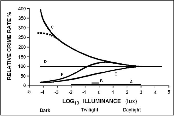
Figure 6. Notional curves for the variation of crime with ambient light. Line A indicates the illuminance range in which lighting and crime experiments are usually performed. The illuminance from a full moon would be a little to the right of –1 on the horizontal axis. Line B represents a 3.375 times increase in light as a typical treatment in experiments. Curve C represents the situation in which crime increases as the ambient light becomes dimmer, as is widely (and wrongly) believed. Line D represents the case where crime is completely independent of ambient light. Curve E is the simplest form of variation implied by the observations of low crime values in blackouts. Curve F is an attempt to reconcile conflicting claims about the form of variation of crime with ambient light.
FIGURE 7. UCR Crime Rate and Upward Light Energy Loss in USA Cities
Figure 7. Crime rate in 1998 for 21 cities in the USA, plotted as a function of annual upward light energy loss per unit area derived from satellite observations in 1997. The light energy loss data are from Isobe and Hamamura (1998). Crime rate data for 1998 are from FBI (1998), with missing data from FightCrimeFortWayne (1999). The regression line slope is not significantly different from zero. Numerical data are in Table 5.
FIGURE 8. Population and Upward Light Energy Loss in USA Cities

Figure 8. Population and annual upward light energy loss for 21 USA cities. Numerical data are in Tables 5 and 6. The top right data point is for New York City. From the right, the three outlier points between 130 and 60 on the light loss scale are for Minneapolis, St Louis and Kansas City MO, each of which had snow cover at the time of satellite observation.
FIGURE 9. UCR Crime and Upward Light Energy Loss per Person in USA Cities
Figure 9. UCR Index Crime Rate for 21 USA cities plotted against annual upward light energy loss per person derived from satellite observations in 1997 (Isobe and Hamamura 1998), with estimated corrections to no-snow conditions for Minnesota, St Louis, Kansas City MO, Buffalo and Denver. The regression line slope is reliably different from zero (p < 0.05). Corresponding numerical data, without and with the corrections for snow, are in Tables 5 and 6.
FIGURE 10. Crime Score and Upward Light Energy Loss per Person in USA Cities

Figure 10. Morgan Quitno (2000) crime score for 21 of 315 USA cities, plotted against annual upward light energy loss per person. The crime score is based on 1998 UCR crime data weighted according to the threat assessed by survey. The mean crime score for the 315 cities is represented by the ordinate value 0. Light energy loss data are from Isobe and Hamamura (1998), with estimated corrections to no-snow conditions for Minnesota, St Louis, Kansas City MO, Buffalo and Denver. US cities population data used are from FBI (1998), with missing data from FightCrimeFortWayne (1999). Numerical data are in Tables 5 and 6. The regression line slope is reliably different from zero (p < 0.01).
FIGURE 11. Crime Rate and Upward Light Energy Loss in Canadian Cities
Figure 11. Crime rate in 1999 for nine cities in Canada, plotted against annual upward light energy loss per unit area measured by satellite in 1997. Light energy loss data are from Isobe and Hamamura (1998). Crime data for 1999 have been calculated from 2000 data from Statistics Canada (2001). Numerical data are given in Table 7. No corrections are made for snow cover. The unfilled data point is for Trois Rivières, which is excluded from the linear regression analysis as an outlier. The slope of the regression line is not significantly different from zero. Including Trois Rivières makes the regression line slope slightly negative, but again not reliably different from zero.
FIGURE 12. Crime and Upward Light Energy Loss per Person in Canadian Cities
Figure 12. Crime rate in 1999 for nine cities in Canada, plotted against annual upward light energy loss per person. Light loss data are from Isobe and Hamamura (1998). Crime data for 1999 have been calculated from 2000 data from Statistics Canada (2001). Numerical data are given in Table 7. No corrections are made for snow cover. The slope of the regression line is not significantly different from zero.
FIGURE 13. Crime and Upward Light Energy Loss in UK Cities
Figure 13. Crime rate in 2000 for 12 UK cities, plotted against annual upward light energy loss measured by satellite in 1997 (Isobe and Hamamura 1998). The English crime rates for 2000 are based on 1991 census data (Povey and Cotton 2000, Povey et al. 2001). Details are given in Table 8. The three crossed data points are for cities in Scotland, with 2001 crime rates based on 2000 population data (Scottish Executive 2002). They are not included in the regression analysis. The slope of the regression line for the nine English cities is reliably different from zero (p < 0.05).
FIGURE 14. Crime and Upward Light Energy Loss in Australian Cities
Figure 14. Crime rate in 2000 or 2000-2001 for seven Australian cities, plotted against annual upward light energy loss measured by satellite in late 1996 (Isobe and Hamamura 1998). Population data are either from ABS (2003) or from the crime data sources, ACT (2002a,b), BOCSAR (2002), OCS (2002), OESR (2002), Vicpol (2002a,b), and WAPS (2002). Numerical data are given in Table 9. The slope of the regression line is not reliably different from zero.
FIGURE 15. Drugs Crime and Light in Bourke Street

Figure 15. Arithmetic means of north and south footpath horizontal plane illuminances for street numbers along Bourke Street, Melbourne, at night in July 2002. The vertical scale is logarithmic. The triangle symbols show the street numbers recorded by police in serious drug offence arrests for the year 2000 (redrawn from Figure 7.10a of DCPC 2001). The large peak near number 150 is from the brightly lit entrance of a hostel and that at 260 is from an intensely lit billboard covering about 7 storeys on a corner building. Typically, streetlights contribute less than 10 lux to the totals (1 on the vertical scale). Intersections have multiple streetlights. The bulk of the light between intersections comes from awning lights, shop windows, escaping indoor light, advertising signs and decorative lighting. The intersection with Russell Street is between numbers 174 and 180: there were no arrests at or close to this gap. Individual shops predominate along Bourke Street to about number 300, followed by major department stores and then an increasing number of office blocks. The street side ambiguity prevents definite identification, but some of the crime locations appear to be near fast-food places that have bright internal and external lighting. Most of the others appear to be near brightly lit shops or bright shop window displays. Bourke Street, with 17 174 recorded crimes including drugs crime from 1995 to 2000, was the city’s most prevalent location for recorded crimes. A little further east (to the left on the horizontal axis) from numbers 1 and 2 is Parliament House, floodlit to about 115 lux (over 2 on the vertical scale), measured in the vertical plane.
FIGURE 16. Drugs Crime and Light in Russell Street
Figure 16. Arithmetic means of east and west footpath horizontal plane illuminances for street numbers along Russell Street, Melbourne, at night in July 2002. The vertical scale is logarithmic. The triangle symbols show the street numbers recorded by police in serious drug offence cases for the year 2000 (redrawn from Figure 7.10b in DCPC 2001). The peak near number 130 is from the intensely lit awning of a motion picture theatre, but two-thirds of those lights are switched off after midnight. The intersection with Bourke Street is between numbers 147 and 152. The elevated light levels between 153 and 233 are from several sources of light in the vicinity, including amusement parlour lighting, advertising signs and ad hoc footpath lighting presumably intended to deter crime. The lighting peaks at about 75, 235 and 333 are near the intersections with Collins Street, Lonsdale Street and Latrobe Street respectively. From 240 onwards the frontages are predominantly building sites and large buildings that are closed at night or unoccupied. Extensive graffiti was noticed on a shop window shutter lit to 11 lux (vertical) in the cross street (Victoria Street) beyond number 380.
[END OF DOCUMENT]